Unraveling the mysteries of Antarctic ice-shelf melting


An aerial view of the edge of the Ross Ice Shelf.
(Photo by Andy Myatt/Alamy.)
Antarctica remains one of Earth’s great enigmas: a frozen continent whose vast white expanse hides many secrets of our planet’s climate. At the continent’s fringes lie the ice shelves, immense floating extensions of the Antarctic Ice Sheet. Those shelves, mapped in figure 1 , act as natural buttresses that hold back the massive inland ice sheets and slow their flow into the ocean. If the entire Antarctic Ice Sheet were to melt, global sea level would rise by about 58 meters 1 and inundate coastlines worldwide. Despite decades of research and exploration, the stability of ice shelves remains uncertain. 2 , 3 Scientists are still grappling with a central question: What controls the rate at which ice shelves melt?
Figure 1.

Major ice shelves on the Antarctic coastline. Regions in red are decreasing in thickness; regions in green are increasing.
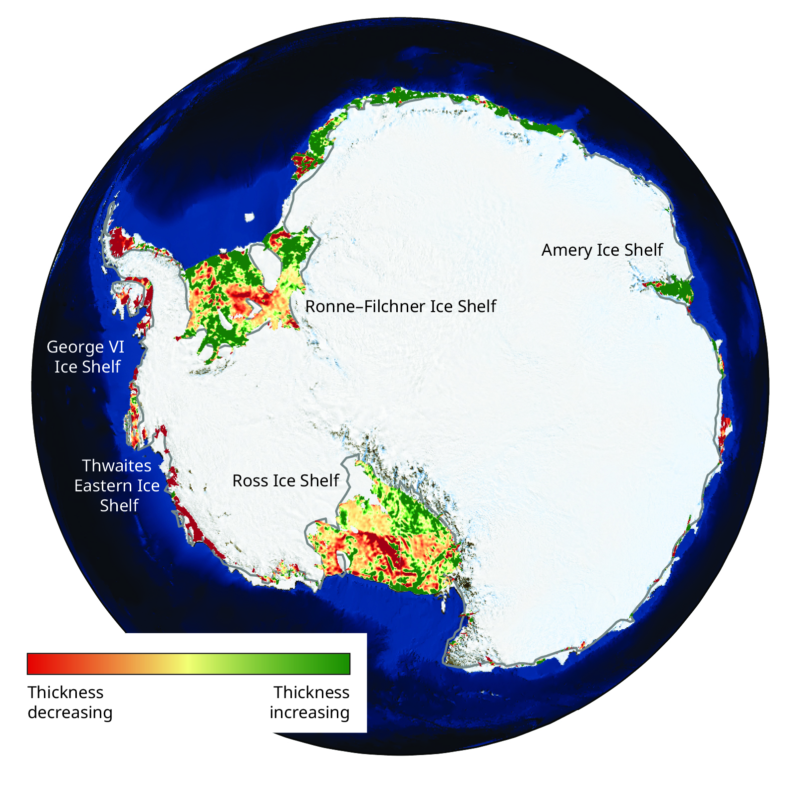
Although the southernmost continent’s ice shelves are colossal—they can stretch across hundreds of kilometers and plunge several kilometers deep—they are thinning and retreating in many locations. They lose mass both by calving icebergs and, more insidiously, by melting from below. 4 That basal melting occurs in the hidden ocean cavities beneath the ice shelves, where glacial ice meets seawater that is warm and salty enough to erode it. The interactions there between the ice and seawater generate complex, turbulent boundary layers that control the flow of heat and salt. The cavities are some of the most intriguing frontiers in polar science and are only now beginning to yield their secrets.
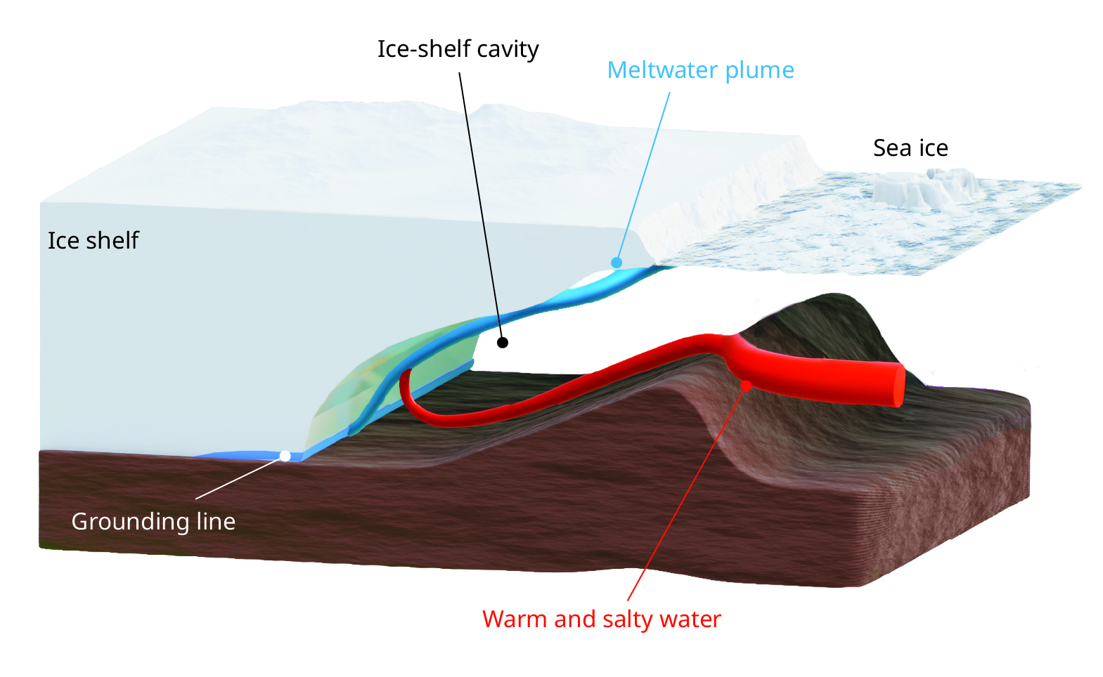
When ice shelves melt from below, as seen in figure 2 , they cool and freshen the ocean—that is, make it less salty. The buoyant meltwater plays a far-reaching role in shaping the Southern Ocean and, ultimately, the global climate. As it spreads outward, it alters the ocean’s temperature, salinity, and density and modifies circulation patterns that extend thousands of kilometers away from Antarctica. Recent studies have assessed how much melting is already unavoidable because of warming caused by past greenhouse gas emissions. 5 But projections of ice-shelf mass loss and meltwater remain highly uncertain: They are hindered by our limited knowledge of the ice–ocean boundary layer, where ocean turbulence and density stratification govern the pace of melting and ultimately affect the fate of rising seas.
The ocean beneath ice shelves
The fate of Antarctic ice is determined not just by large-scale climate forcing but by what happens in a much narrower area within boundary layers typically just several millimeters to a few centimeters thick beneath the ice shelves. 6 , 7 In those boundary layers, temperature and salinity gradients regulate how heat and salt diffuse and are exchanged between the ocean and the ice. The transfer of saltier water toward the base of an ice shelf causes melting to occur more rapidly; the presence of salt decreases the temperature at which ice melts, so saltwater is warmer relative to its freezing point than is freshwater at the same temperature. Because heat diffuses roughly 100 times as fast as salt, their gradients are markedly different: A thicker thermal boundary layer overlies a thinner salinity boundary layer just beneath the base of an ice shelf. That asymmetry establishes strong buoyancy gradients that determine whether the local stratification—the natural separation of seawater into layers of differing density—is stable or unstable.
Figure 2.

A schematic view of an Antarctic ice- shelf cavity. At bottom left is the grounding line, the boundary between ice resting on bedrock and the floating ice shelf. Melting at the bottom of the shelf can produce meltwater plumes (blue), which draw in warmer and saltier water (red) circulating in the Southern Ocean.
Boundary-layer turbulence is governed by the buoyancy differences in seawater, which arise from variations in temperature and salinity and generate or suppress motion depending on the stability of the stratification. An unstable buoyancy profile, in which denser fluid lies above lighter fluid, drives overturning motion and forms turbulent convective plumes that vigorously mix the surrounding water. But a stable buoyancy profile, in which lighter water overlies denser water, resists vertical motion and suppresses turbulence. The shifting balance between buoyancy-driven convection and buoyancy-suppressed turbulence in the water beneath an Antarctic ice shelf dictates how effectively heat is carried to the ice shelf’s base and, ultimately, how fast the ice melts.
The velocity boundary layer impacts the local generation or suppression of turbulence in the ocean flow. Immediately beneath the ice, the ocean flow experiences the ice face as a solid boundary that exerts frictional drag, which shapes the velocity field.
The velocity boundary layer can be decomposed into distinct regions, as seen in figure 3 . Closest to the ice is a millimeter- to centimeter-thick viscous sublayer, where the flow motion is extremely weak and momentum transport is dominated by viscosity. It encompasses the temperature and salinity boundary layers, in which heat and salt travel only by diffusion, and is critical to the exchange process between ocean and ice.
Figure 3.

The ocean layers underneath an Antarctic ice shelf. The velocity boundary layer, in which momentum exchange takes place, encompasses three layers: the viscous sublayer, the shear layer, and the outer layer. Immediately below the ice is the viscous sublayer, a few millimeters to centimeters thick, where flow is extremely weak. It encompasses the temperature and salinity boundary layers, in which heat and salt exchange takes place. Below that is the shear layer, approximately a few meters thick, which forms when the current is sufficiently strong. That is followed by the outer layer, on the order of tens of meters thick, where the flow is still partially governed by the presence of the ice. Below that is the far-field ocean, which is unaffected by the overlying ice shelf.
(Ice texture adapted from iStock.com/rusm.)
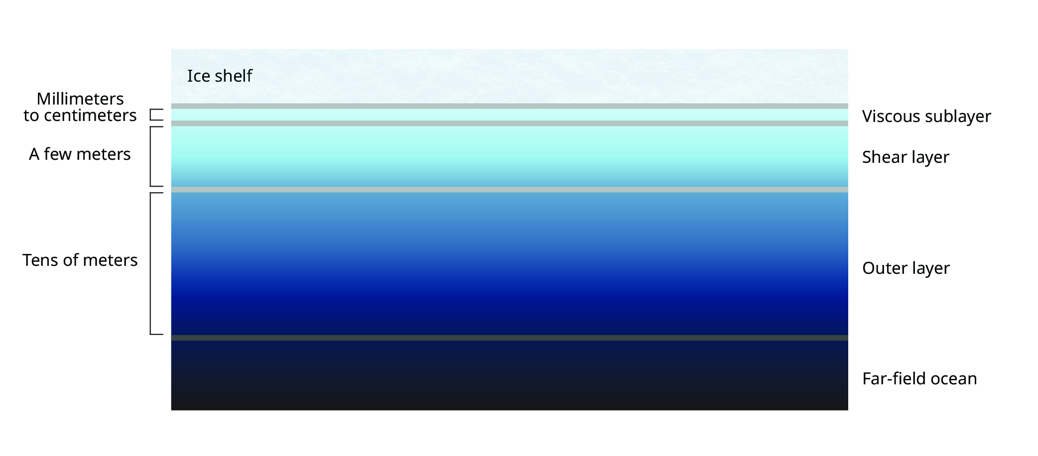
Beneath the viscous sublayer lies a meter-scale shear layer, which exists only when the current is strong enough to generate significant shear in the velocity boundary layer. In the shear layer, the velocity increases rapidly with distance from the ice, a consequence of the drag that the ice exerts on the flow.
Extending tens of meters deeper is the outer layer, in which Earth’s rotation bends the direction of the current, but the flow is still partially governed by the presence of the ice. Beyond that layer lies the far-field ocean, in which the flow is largely unaffected by the overlying ice.
Regimes of ice-shelf melting
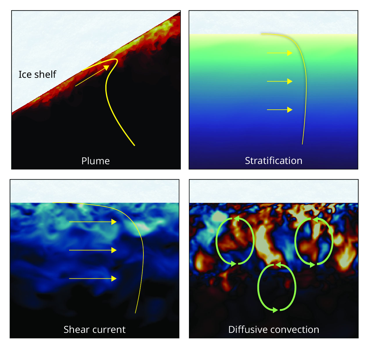
A melting ice shelf not only responds to the surrounding ocean flow in the velocity boundary layer but also organizes that flow. As ice melts, it releases cold, fresh meltwater, which makes the water immediately beneath the ice more buoyant than the ocean layers below. Depending on the slope of the ice shelf and the strength of the ocean currents, that buoyancy difference can either destabilize or stabilize the flow. Our present understanding of the ocean dynamics under ice shelves reveals four distinct flow regimes, presented in figure 4 , that develop when shelves melt: plume, stratification, shear current, and diffusive convection.
The fate of Antarctic ice is determined not just by large-scale climate forcing but by what happens in a much narrower area within boundary layers typically just several millimeters to a few centimeters thick beneath the ice shelves.
When the base of an ice shelf is sloped—near, for example, the grounding line, where the ice, ocean, and seafloor meet—the buoyant meltwater rises along the slope, forming a plume, as seen in the top-left panel of figure 4 . The melt-induced buoyancy initially drives small, irregular motions that then organize into convective plumes, which draw in warmer, saltier water from farther away and move it toward the ice. In the plume regime, convection continuously draws heat to the ice interface and sustains and amplifies melting. Because meltwater plumes are large and slow moving, they are difficult to observe. But possible plume signatures have been detected under the Ross Ice Shelf, among other locations. 8
When the base of an ice shelf is roughly horizontal, the buoyant meltwater tends to pool beneath the ice, which creates a stably stratified layer that suppresses vertical flow motion, as seen in the top-right panel of figure 4 . In the stratification regime, the amount of heat reaching the ice is largely determined by external flows, such as tides, that generate shear and turbulence. Those external flows can move warm water toward the ice, which increases melting. But as has been observed beneath the Thwaites Eastern Ice Shelf, 9 strong stratification can also dampen turbulence in the shear layer, which effectively insulates the ice and slows its loss. The result is a dynamic balance, in which buoyancy, current shear, and turbulence interact to dictate the local rate of melting.
When the current flow is sufficiently strong, as seen in the bottom-left panel of figure 4 , turbulence is fully driven by shear and buoyancy is only passive. In that scenario, termed the shear-current regime, the velocity boundary layer becomes well mixed, and temperature and salinity gradients are largely erased by vigorous turbulent motions. Heat and momentum are transported efficiently across the layer, which maintains nearly uniform temperature and salinity profiles up to the base of an ice shelf. The shear-current regime can typically be found in energetic, cold cavities, such as the cavity beneath the Larsen Ice Shelf, in which strong inflows and tides overwhelm buoyancy effects close to the ice base. 10
In quiescent regions with shallow ice slopes and minimal ocean flow, the diffusive-convection regime—shown in the bottom-right panel of figure 4 —governs ice-shelf melting. Because heat diffuses about 100 times as fast as salt, two separate layers form next to the ice: a thicker thermal boundary layer and a thinner salinity boundary layer. That imbalance creates small but persistent diffusive convection, in which cooler, denser water near the ice forms gentle downward plumes that mix with the slightly warmer, saltier water below. As observed beneath the George VI Ice Shelf, 11 the result is a series of double-diffusive layers, each typically a few meters to tens of meters thick, in which heat and salt slowly diffuse at different rates toward the ice. Although those layers are weaker than the convective plumes in the plume regime, they can still enhance melting above what would occur through diffusion alone.
Figure 4.

The four regimes of ice-shelf melting. Yellow lines indicate the profile of ocean flow; yellow arrows, relative flow velocity; and green arrows, diffusive convection. In the plume regime, buoyant meltwater forms a plume and rises along a sloped segment of the ice shelf. In the stratification regime, buoyancy acts to increase stable stratification, suppress turbulence, and moderate the melt rate. In the shear-current regime, temperature and salinity gradients are largely erased by vigorous turbulent motions. In the diffusive-convection regime, a series of double-diffusive layers slowly transport heat and salt toward the ice at different rates and increase the melt rate.
(Ice texture adapted from iStock.com/rusm.)
Both the plume and diffusive-convection regimes result in an enhanced melting rate because the buoyancy differences in those regimes generate flow, increase turbulence, and boost the rate at which heat and salt are supplied to the ice. In contrast, the shear-current regime has weak buoyancy effects, which generally do not affect the flow turbulence. And in the stratification regime, buoyancy acts to increase stable stratification, which suppresses turbulence and moderates the melt rate.
Some regions are not easily categorized into one regime. A region can oscillate between the stratification and shear-current regimes, for example, when tides cause the flow speed to change. Other ocean dynamics, including the formation of marine ice—seawater frozen into small crystals or directly onto the ice base—also influence the flow dynamics and melt rate. Researchers are currently attempting to improve our understanding of the effects of ocean dynamics in those more complex cases.
Revealing hidden boundary layers
Obtaining direct observations of ocean cavities beneath Antarctic ice shelves is one of the great difficulties of polar research. The cavities are vast and remote, and they lie under hundreds to thousands of meters of ice, which makes accessing them both technically demanding and hazardous. Despite those obstacles, researchers have made remarkable progress over the past decade in directly observing the ice–ocean boundary layer.
Historically, most data on ocean cavities came from ships near the edges of ice shelves. The ships provided valuable information on ocean waters entering and exiting the cavities. Starting in the 1960s, satellite measurements began helping researchers infer ice-shelf extent and thickness. But the real breakthrough came in the late 1970s, with the development of borehole drilling. Using hot-water drills, scientists can now melt narrow access holes—typically just tens of centimeters wide—all the way through the ice and insert instruments beneath the shelf. Offering the first in situ view of processes at the ice base, borehole studies measure local melt rates, turbulence properties, temperature, salinity, and small-scale ice topography.
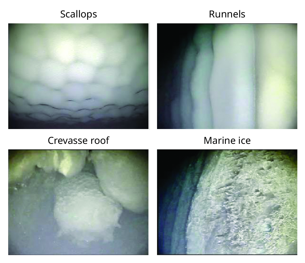
Figure 5.

Images of topographical ice features in the base of the Ross Ice Shelf taken by the remotely operated underwater vehicle Icefin. The top two images show scallops and runnels on the top of the ice-shelf cavity. At bottom left is an image of the roof of a crevasse in an ice-shelf cavity, and at bottom right is an image of marine ice: seawater that has frozen directly onto the top of the ice-shelf cavity.
(Images adapted from ref. 12.)
In recent years, autonomous vehicles, such as the remote-controlled underwater robot Icefin, have enabled measurements to be taken across wide swaths of the ocean cavities (for more on Icefin, see the April 2023 PT article “Melting underneath Thwaites Glacier is more complicated than expected ”). They are able to reach dynamically important regions near the grounding line. 12 Those missions have revealed how the ice base’s rich topography, four examples of which are shown in figure 5 , can change dramatically over just a few meters. Those differences hint at the flow dynamics present in the boundary layers. 12 , 13
Given that observations of ice–ocean interactions remain difficult to obtain, researchers have developed a hierarchy of modeling approaches to complement them. Large-scale and regional ocean models simulate the circulation in ice-shelf cavities and capture the interactions of meltwater and currents. But those models cannot resolve the thin, turbulent boundary layers that control melting. Instead, they parameterize small-scale processes by using simplified 1D formulations. The widely used three-equation model, for example, links the melt rate to local differences in temperature and salinity between the ocean and the ice by solving coupled equations for heat balance, salt balance, and the interface temperature. 14 , 15
Because our knowledge of the underlying physics remains incomplete, formulations like the three-equation model contain large uncertainties. To improve our understanding, scientists have begun using state-of-the-art laboratory experiments and boundary-resolving simulations that explicitly capture the flow and turbulence near the ice base. Laboratory studies of ice melting in seawater date back more than four decades and re-main invaluable for exploring meltwater plumes, double-diffusive layering, and the interplay of buoyancy, turbulence, and rotation. 16 Today’s experiments, often conducted in cold rooms or on rotating tables, allow researchers to track ice-face evolution, measure turbulence, and visualize flow structures at millimeter resolution. 6 They are complemented by numerical simulations that can resolve the thin boundary layers and turbulent plumes responsible for heat and salt transfer.
Those approaches often use principles of dynamical similarity to infer the ocean-cavity dynamics. Both experiments and numerical simulations are crucial for revealing the fundamental balances in the boundary layer and for identifying the distinct melting regimes observed around Antarctic ice shelves. They provide insights that can help improve the simplified parameterizations used in larger-scale ocean models.
When combined, observations, laboratory experiments, and boundary-resolving numerical simulations provide a pathway toward obtaining an accurate picture of melt rate, which is crucial to improving projections of sea-level rise. As each new generation of instruments and models brings us closer to resolving the turbulent boundary layer in detail, the once-inaccessible world beneath Antarctica’s ice shelves is gradually coming within reach.
New frontiers
Recent advances in observations, laboratory studies, and modeling are finally illuminating the turbulent boundary layer where Antarctic ice shelves meet the ocean. Those efforts reveal how buoyancy, shear, and stratification interact to shape the many regimes of melting that govern the stability of the ice shelves. Improving our understanding of those regimes, each of which responds differently to currents, stratification, and buoyancy, offers a pathway to improve how large-scale models represent ice-shelf melting so that simulations more closely align with real-world observations.
Obtaining direct observations of ocean cavities beneath Antarctic ice shelves is one of the great difficulties of polar research. The cavities are vast and remote, and they lie under hundreds to thousands of meters of ice, which makes accessing them both technically demanding and hazardous. Despite those obstacles, researchers have made remarkable progress over the past decade in directly observing the ice–ocean boundary layer.
The next frontier in Antarctic ice-shelf research lies in uniting those diverse approaches into an integrated Earth-system framework. New coupled atmosphere-ocean-ice models, informed by laboratory and field measurements, are beginning to illustrate how surface winds, sea-ice loss, and turbulent boundary layers interact to control basal melting. And scientists are working toward the development of models that link boundary-resolving simulations, which explicitly capture the fine-scale turbulence and melt processes, with large-scale ocean models that simulate cavity-wide circulation. Running those models side by side would help us better understand how small-scale physics informs global climate behavior.
Understanding ice-shelf melting is critical to modeling the future behavior of the Antarctic Ice Sheet: When ice shelves thin, they weaken and become unable to fully buttress the grounded ice sheets they are holding back. As a result, inland ice flows into the ocean and increases sea levels. 17 Global climate models currently struggle to simulate how ice-shelf melting affects the stability of inland ice sheets. Coupling models of ice-sheet dynamics with models of the ocean and atmosphere is a key, albeit difficult, step toward improving projections of climate change and sea-level rise. 18
Meanwhile, advances in robotics and machine learning are enabling autonomous vehicles to collect and interpret sub-ice data in near real time. Interdisciplinary teams will be needed to stitch all the approaches together to better understand the underlying physics and the climate impact (see the June 2021 PT article “Accelerating progress in climate science ,” by Tapio Schneider, Nadir Jeevanjee, and Robert Socolow).
Together, those innovations are moving us closer to the point at which we will be able to accurately predict the stability of Antarctic ice shelves, which is crucial to projecting the pace of global sea-level rise in a warming world.
Catherine A. Vreugdenhil is supported by an Australian Research Council Discovery Early Career Researcher Award, grant number DE220101027. Both authors appreciate the support of the Australian Research Council Discovery Project (grant number DP240102823) and the Australian Centre for Excellence in Antarctic Science (project number SR200100008). Numerical simulations were performed on the National Com-putational Infrastructure at the Australian National University in Canberra. For valuable discussions and assistance in creat-ing the figures, the authors thank Bajrang Chidhambarana-than, Kaushik Mishra, Madelaine G. Rosevear, Benjamin K. Galton-Fenzi, Taimoor Sohail, Peter Washam, and John R. Taylor.
References
1. M. Morlighem et al., “Deep glacial troughs and stabilizing ridges unveiled beneath the margins of the Antarctic Ice Sheet ,” Nat. Geosci. 13, 132 (2020).
2. N. J. Abram et al., “Emerging evidence of abrupt changes in the Antarctic environment ,” Nature 644, 621 (2025).
3. H. A. Fricker et al., “Antarctica in 2025: Drivers of deep uncertainty in projected ice loss ,” Science 387, 601 (2025).
4. C. A. Greene et al., “Antarctic calving loss rivals ice-shelf thinning ,” Nature 609, 948 (2022).
5. K. A. Naughten, P. R. Holland, J. De Rydt, “Unavoidable future increase in West Antarctic ice-shelf melting over the twenty-first century ,” Nat. Clim. Change 13, 1222 (2023).
6. Y. Du, E. Calzavarini, C. Sun, “The physics of freezing and melting in the presence of flows ,” Nat. Rev. Phys. 6, 676 (2024).
7. M. G. Rosevear et al., “How does the ocean melt Antarctic ice shelves? ,” Annu. Rev. Mar. Sci. 17, 325 (2025).
8. C. Stevens et al., “Ocean mixing and heat transport processes observed under the Ross Ice Shelf control its basal melting ,” Proc. Natl. Acad. Sci. USA 117, 16799 (2020).
9. P. E. D. Davis et al., “Suppressed basal melting in the eastern Thwaites Glacier grounding zone ,” Nature 614, 479 (2023).
10. P. E. D. Davis, K. W. Nicholls, “Turbulence observations beneath Larsen C Ice Shelf, Antarctica ,” J. Geophys. Res. Oceans 124, 5529 (2019).
11. S. Kimura, K. W. Nicholls, E. Venables, “Estimation of ice shelf melt rate in the presence of a thermohaline staircase ,” J. Phys. Oceanogr. 45, 133 (2015).
12. P. Washam et al., “Direct observations of melting, freezing, and ocean circulation in an ice shelf basal crevasse ,” Sci. Adv. 9, eadi7638 (2023).
13. A. Wåhlin et al., “Swirls and scoops: Ice base melt revealed by multibeam imagery of an Antarctic ice shelf ,” Sci. Adv. 10, eadn9188 (2024).
14. D. M. Holland, A. Jenkins, “Modeling thermodynamic ice–ocean interactions at the base of an ice shelf ,” J. Phys. Oceanogr. 29, 1787 (1999).
15. M. S. Dinniman et al., “Modeling ice shelf/ocean interaction in Antarctica: A review ,” Oceanography 29, 144 (2016).
16. H. E. Huppert, J. S. Turner, “Ice blocks melting into a salinity gradient ,” J. Fluid Mech. 100, 367 (1980).
17. T. L. Noble et al., “The sensitivity of the Antarctic Ice Sheet to a changing climate: Past, present, and future ,” Rev. Geophys. 58, e2019RG000663 (2020).
18. R. S. Smith et al., “Coupling the U.K. Earth system model to dynamic models of the Greenland and Antarctic Ice Sheets ,” J. Adv. Model. Earth Syst. 13, e2021MS002520 (2021); D. T. Bett et al., “Coupled ice–ocean interactions during future retreat of West Antarctic ice streams in the Amundsen Sea sector ,” Cryosphere 18, 2653 (2024).
More about the authors
Catherine A. Vreugdenhil is a senior lecturer in the department of mechanical engineering at the University of Melbourne in Australia and a chief investigator with the Australian Centre for Excellence in Antarctic Science. Her research focuses on the modeling of Antarctic ice shelf–ocean interactions and ocean circulation.
Bishakhdatta Gayen is an associate professor in the department of mechanical engineering at the University of Melbourne in Australia and a chief investigator with the Australian Centre for Excellence in Antarctic Science. He is also an assistant professor at the Centre for Atmospheric and Oceanic Sciences at the Indian Institute of Science in Bengaluru. His research focuses on the modeling of Antarctic ice shelf–ocean interactions and ocean circulation.


