New Algorithm Speeds Up Computer Simulations of Complex Fluids
DOI: 10.1063/1.1712490
In a colloidal dispersion, particles much bigger than atoms are spread more or less uniformly amid a molecular fluid. Paint is a colloidal dispersion; so are ice cream, smog, and shampoo.
Less quotidian are the myriad new colloids being developed for drug delivery, photonics, and other high-tech applications. Materials scientists like the colloid concept because it combines functional nanoparticles, whose aggregate surface is huge, with a supporting medium, whose properties can be tailored and transformed.
Predicting and optimizing a colloid’s properties requires a physical model. But the colloid’s mix of particle sizes, along with the range and variety of forces present, frustrates the modeler. Even though one can write down exact equations for the interparticle forces, obtaining a solution for the bulk substance is impossible without severe approximations. Numerical approaches founder under the colossal computational load.
Now, Erik Luijten of the University of Illinois at Urbana-Champaign and Jiwen Liu, his graduate student, have devised a new simulation algorithm. 1 Thanks to its exquisite efficiency, Luijten and Liu’s algorithm can tackle fluid systems, like the colloids shown in figure 1, that were once all but impossible to simulate.

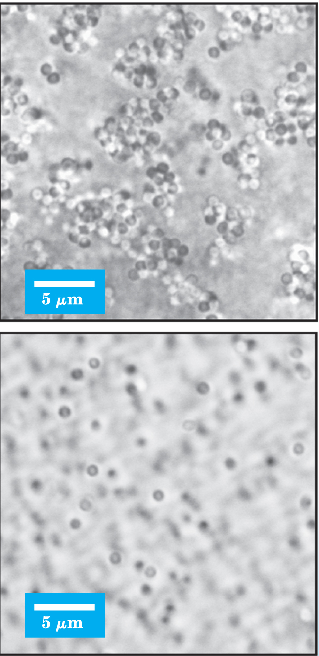
Figure 1. These colloidal suspensions consist of silica microspheres in dilute nitric acid. Because of Van der Waals attractions, the microspheres tend to clump together, as shown in the top panel. Adding charged nanospheres, as shown in the bottom panel, prevents the clumping.
(Adapted from ref. 7.)
Movies and snapshots
To understand why simulating certain fluid systems is so difficult, consider what might seem the most obvious approach. First, construct a trial configuration and note the initial positions and velocities of all the constituent particles. Calculate the forces acting on each particle, apply Newton’s second law of motion, and then determine where the particles end up after an incremental step in time. Repeat as necessary.
This approach, known as molecular dynamics (MD), yields what can be thought of as a movie of the system—that is, a time-ordered sequence of stills, each of which captures an instantaneous state of the system and which is connected to its neighbors by physical dynamics.
Even with a supercomputer, MD can track a typical condensed matter system for little more than a millisecond. Although that span may suffice for a fluid of identical particles, it’s too short for colloids because the large suspended particles barely move on that timescale. And if one tried to speed up the simulation by taking larger time steps, the crucial behavior of the fluid particles would be missed.
Half a century ago, when computers were 1010 times more feeble than their modern counterparts, physicists developed the probabilistic approaches known collectively as Monte Carlo. Of these, the variant published in 1953 by Nicholas Metropolis and his coworkers has proven to be the most influential and popular. 2
The Metropolis algorithm doesn’t attempt to track every particle. Rather, the simulation proceeds by randomly picking a single particle from a trial configuration and moving it. If the move ends up lowering the system’s energy, the new configuration is accepted. If the move raises the energy, the new configuration is accepted with a probability of exp(−ΔE/kT).
Moving only one particle at a time is unphysical, but the Metropolis acceptance criterion ensures that the set of accepted configurations converges to thermodynamic equilibrium. The algorithm also ensures that the accepted configurations represent the most frequently occupied states, rather than a random sampling of all possible states. Without that key property, the algorithm would be useless.
So, if MD is like a movie, the Metropolis algorithm is like a sparse set of shuffled snapshots. If you simulated a cocktail party with the Metropolis algorithm, you wouldn’t see dynamical events, such as guests arriving and departing, or rare events, such as a waiter refilling a punchbowl. But, taken together, the Metropolis snapshots would fairly represent the party in full swing. From them, you could deduce whether, on average, people had enjoyed themselves.
The Metropolis algorithm is one of the most widely used and crops up in such diverse fields as banking and astrophysics. But like MD, it’s stumped by colloidal systems. The difficulty lies in the big particles, which can’t be lifted and repositioned without dislodging smaller particles at high energetic cost.
Before Luijten and Liu’s algorithm cracked the fluid problem, other workers had shown how to make the Metropolis algorithm work in another difficult arena: spin lattices close to critical points.
A digression on spin lattices
The Ising model of ferromagnetism is among the most studied systems in statistical physics. Each site in a notional lattice is occupied by a spin that can point up or down, with a tendency to align both with its neighbors and with an external magnetic field.
At high temperatures, the spins have more than enough energy to break out of alignment, and each spin flips between the two states with high probability. At low temperatures, the spins still flip, albeit less readily, but alignment prevails and only individual, sporadic flips occur.
Despite its simplicity, the Ising model can’t be solved analytically in three dimensions. But it’s almost perfectly framed for the Metropolis algorithm—except, that is, in the vicinity of a critical point.
When the temperature of an Ising system drops toward the Curie temperature, large-scale fluctuations emerge. Flipping spins one at a time à la Metropolis fails to follow the fluctuations. The closer the system approaches this critical point, the more moves are needed to reach a new, uncorrelated state. Like a car vainly spinning its wheels in a muddy ditch, the simulation stops advancing.
In 1987, Robert Swendsen and Jian-Sheng Wang of Carnegie Mellon University found a way to dispose of this so-called critical slowing. 3 Rather than flip one spin per move, they flip several at once and in such a way that the entire move is guaranteed acceptance.
To identify which spins to flip, Swendsen and Wang exploited a mathematical mapping devised in the late 1960s by Piet Kasteleyn and his graduate student, Cees Fortuin. 4 In that mapping, spin–spin interactions are recast as bonds whose strength depends on the degree of alignment. Temperature and energy also contribute to bond strength.
Swendsen and Wang realized the bound spins form clusters that could be flipped en bloc. Their algorithm can sail through a critical point without stopping. Its clusters even correspond, more or less, to the large-scale fluctuations that form and percolate around a critical point.
Geometric clusters
The Swendsen–Wang algorithm, and its refinement by Ulli Wolff two years later, 5 revolutionized the study of lattice spin systems. But when modelers sought to adapt the cluster approach to fluids, they hit a problem. The Swendsen–Wang algorithm succeeds, in part, because of an intrinsic symmetry: Flipping a spin twice recovers the original state. That convenient restoration doesn’t happen when a fluid particle undergoes two identical displacements.
In 1995, Werner Krauth and Christophe Dress of the Ecole Normale Supérieure in Paris realized that a messy, disordered fluid does have a symmetry of sorts. Reflecting a particle twice about a point returns the particle to its starting point.
Of course, a reflection is hardly independent of its original state. However, as Krauth and Dress showed, reflection can help identify clusters of particles that can be moved without incurring rejection.
To grasp the basic idea, consider a two-dimensional system in which all the particles have the same size. Start with a trial configuration A. Pick a point within A at random and rotate A about it by 180° to produce a new configuration B (in 2D, rotating the configuration by 180° is equivalent to reflecting individual particles). Superpose A and B to make C.
Now, examine C. Any particle that has an overlap in C can be moved from its position in A to the position it has in B without bumping into another particle. Provided the interparticle forces are sufficiently short-ranged, such a move won’t incur a rejection-triggering increase in energy. The group of translated particles makes up the cluster, and the resulting new configuration is a mix of those particles that moved through a 180° rotation and those that stayed put. 6
Krauth and his coworkers successfully used their geometric cluster algorithm to simulate certain idealized cases, such as the phase separation of big and small hard spheres. But the particle interactions in colloids and other fluid systems are long-ranged. To adapt their algorithm to realistic systems, Krauth and company added an extra round of acceptance tests. Applying those tests led to too many rejections.
General geometric cluster
Luijten and Liu provided the missing ingredient. Like Krauth and Dress, they reflect particles about a randomly selected pivot. But, like Swendsen and Wang, they do so without incurring costly rejections.
Figure 2 illustrates how the algorithm works. First, the algorithm generates a random pivot (the red dot in panel b) and picks a particle (colored yellow and labeled 1) for a point reflection to a new position (colored blue). Any particles that fall under the influence of particle 1, either in its old position or its new position, become candidates to join the cluster.

Figure 2. Erik Luijten and Jiwen Liu’s algorithm takes an initial trial state (a) through a set of reflections (b) to a new state (c).
(Adapted from ref. 1.)
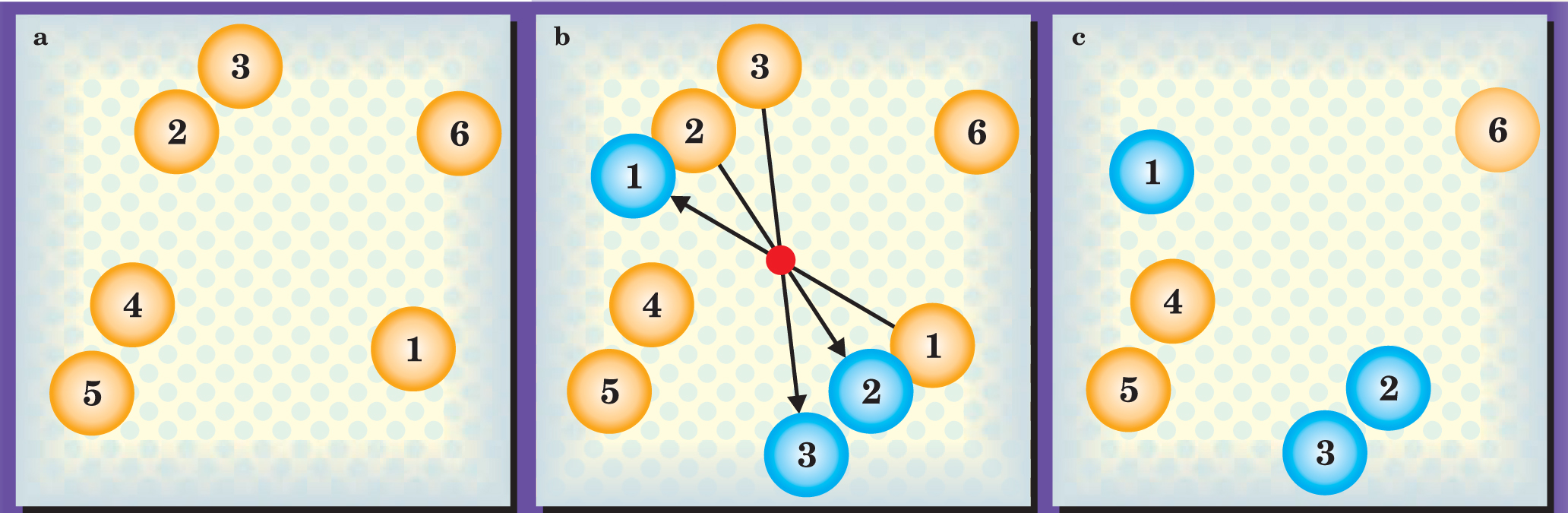
Particle 2, being close to particle 1’s new position, is the first candidate. If, by moving, particle 2 can lower its energy with respect to particle 1 by ΔE, its probability of moving is 1 – exp(−ΔE/kT). That happens to be the case here, so particle 2 undergoes a point reflection about the pivot. If, on the other hand, the move entailed an increase in the pair’s energy, the move would be discarded outright.
Particle 3 is out of range of particle 1’s new or old positions, so the algorithm evaluates particle 3 with respect to particle 2. Because the interparticle force happens to be attractive in this example, particle 3 joins the cluster with high probability, as in figure 2.
Particles 4, 5, and 6 are out of range of the first three particles in their old and new positions, so the cluster stops growing, the algorithm picks a new pivot, and the cluster-building process starts afresh.
Because of symmetry, the interacting particles that form a cluster retain their original separations and energies when they move. But, as figure 2 shows, the cluster’s particles change position relative to the particles that don’t belong to the cluster. After several clusters have moved, the system reaches a configuration that no longer resembles its starting point.
The speed with which an algorithm moves from one uncorrelated state to the next is a key measure of its performance. As the box above shows, certain two-particle mixtures that were impossible to simulate with the Metropolis algorithm are now tractable with Luijten and Liu’s algorithm.
How general is the algorithm? If the colloidal particles are packed too tightly, the algorithm will find only one cluster—the entire system–and won’t be able to reach an uncorrelated state. Luijten estimates the limit is reached when the colloidal particles occupy a quarter of the total volume.
Further limits, applications, and extensions will most likely emerge when other modelers implement the algorithm for themselves. So far, their reaction has been favorable. “It’s brilliant,” said Swendsen. Krauth was even more effusive: “When I read Erik’s paper, I freaked out!”
Energy Autocorrelation Time and Efficiency
The energy autocorrelation time τ measures the time a computer takes to calculate a transition from one state to another whose energy is completely uncorrelated. In a Metropolis simulation, reaching an uncorrelated state always involves several computational steps because successive configurations, being the result of moving a fraction of the particles, tend to be similar. Going from one configuration to the next can also take several steps, especially when trial moves tend to be rejected. Thus, τ provides a measure of an algorithm’s efficiency.
The figure shows how efficiently Erik Luijten and Jiwen Liu’s generalized geometric cluster algorithm and the Metropolis algorithm tackle the same test: determining equilibrium properties of a fluid mixture of two differently sized particles. The big particles repel each other with a Yukawa-style force, whereas the small particles interact with each other and with the big particles like hard spheres.

Both algorithms perform equally well when the big particles are no more than twice the size of the small particles. In that case, the algorithms each consume about a millisecond of CPU time per particle move between uncorrelated states. Given that one typically needs about 10 000 such states to characterize thermodynamic equilibrium, both algorithms are fast.
But look what happens when the size ratio approaches 8. The Metropolis algorithm is unable to reach equilibrium, unlike the geometric cluster algorithm, which is more efficient for all size ratios. (Adapted from ref. .)
References
1. J. Liu, E. Luijten, Phys. Rev. Lett. 92, 035504 (2004).https://doi.org/10.1103/PhysRevLett.92.035504
2. N. Metropolis, A. A. Rosenbluth, M. M. Rosenbluth, A. A. Teller, E. Teller, J. Chem. Phys. 21, 1087 (1953).https://doi.org/10.1063/1.1699114
3. R. R. Swendsen, J.-S. Wang, Phys. Rev. Lett. 58, 86 (1987).https://doi.org/10.1103/PhysRevLett.58.86
4. C. C. Fortuin, P. P. Kasteleyn, Physica (Utrecht) 57, 536 (1972).https://doi.org/10.1016/0031-8914(72)90045-6
5. U. Wolff, Phys. Rev. Lett. 62, 361 (1989).https://doi.org/10.1103/PhysRevLett.62.361
6. C. Dress, W. Krauth, J. Phys. A 28, L597 (1995).https://doi.org/10.1088/0305-4470/28/23/001
7. V. Tohver et al., Proc. Natl. Acad. Sci. USA 98, 8950 (2001).https://doi.org/10.1073/pnas.151063098


