Experiment demonstrates quantum entanglement between atoms a meter apart

The quantum entanglement of spatially separated objects embodies the essence of what’s profoundly weird about quantum theory. Albert Einstein called it spukhafte Fernwirkung (spooky action at a distance). Independent measurements on the two separated objects manifest a degree of correlation that no amount of collusion before the separation could possibly have prearranged. And yet, since the early 1970s experimenters have been creating entangled states that do indeed exhibit the predicted correlation that common sense—as quantified in John Bell’s famous inequality—excludes as impossible. ¹ (See the article by David Mermin in Physics Today, April 1985, page 38 .)

Pioneering tests of Bell’s inequality with entangled photons separated by macroscopic distances were carried out by Stuart Freedman and John Clauser in the 1970s and by Alain Aspect and coworkers in the 1980s. And at distances on the order of microns, entanglement has been studied in pairs of atoms with a view to applications in quantum computing.

Internal states of atoms can coherently store binary quantum-information bits (qubits) for long times. But photons have been the more obvious carriers of quantum information over the macroscopic distances that large-scale quantum computing will probably require. Now Christopher Monroe’s group at the University of Michigan has reported the first observation of entanglement in a pair of trapped single atoms separated by a macroscopic distance. ²

Entangling strangers

A quantum state of two particles is said to be entangled if their joint wavefunction cannot be expressed as a product of two one-particle wavefunctions. An oft-cited example is the decay of a spinless particle into two identical spin-1/2 daughters. But in the new experiment the two entangled atoms did not emerge from a common parent. They’d never even been in contact. So how did they become entangled?

Monroe and company held one singly ionized ytterbium atom in each of two identical ion traps separated by about 1 meter. The ion ¹⁷¹Yb⁺ has a lone valence electron. And the spin of its nucleus, like that of the electronic configuration, is ½. So the ion’s l = 0 S-wave electronic ground state has four different hyperfine substates |F, m〉, where the ion’s total angular momentum F can be 1 or 0, and its projection m along the direction of the 5-gauss magnetic field B applied to both traps can be ±1 or 0.

For the two qubit states with which the group sought to demonstrate entanglement, they chose the S-wave hyperfine substates |1, 0〉 and |0, 0〉, which they label |↑〉 and |↓〉, respectively. Hyperfine substates of the electronic ground state have the virtue of living almost forever—unless they are intentionally disturbed. That makes them particularly attractive for quantum computing and for atomic clocks (see the article by James Camparo on page 33 of this issue).

“Unlike experiments in which atomic qubits are entangled by direct interaction and remain in contact,” says Monroe, “ours is a probabilistic demonstration of entanglement.” in fact, the group found evidence of entanglement only a few times per billion tries. “But we do know when a trial has produced entanglement.” The experiment sought to create what has been called heralded entanglement between ionic states by mingling the photons from the birth of those states.

Once every microsecond, each of the two trapped ions was laser cooled and optically pumped to its S-wave |↓〉 hyperfine ground state, and then both were simultaneously zapped with a polarized picosecond laser pulse intended to excite them to the l = 1 P-wave hyperfine substate |1, −1〉. From that short-lived state, each ion emits a 369.5-nm photon within a few nanoseconds as it decays to one of three S-wave hyperfine states: |↑〉, |↓〉, or |1, −1〉 (see figure 1).

The photon from decay to the un-wanted |1, −1〉 state is distinguishable by its polarization. The other two possible decay photons are distinguishable from each other only by the part-in-10⁵ wavelength difference corresponding to the 12.6-GHz hyperfine splitting between the |↑〉 and |↓〉 qubit states.

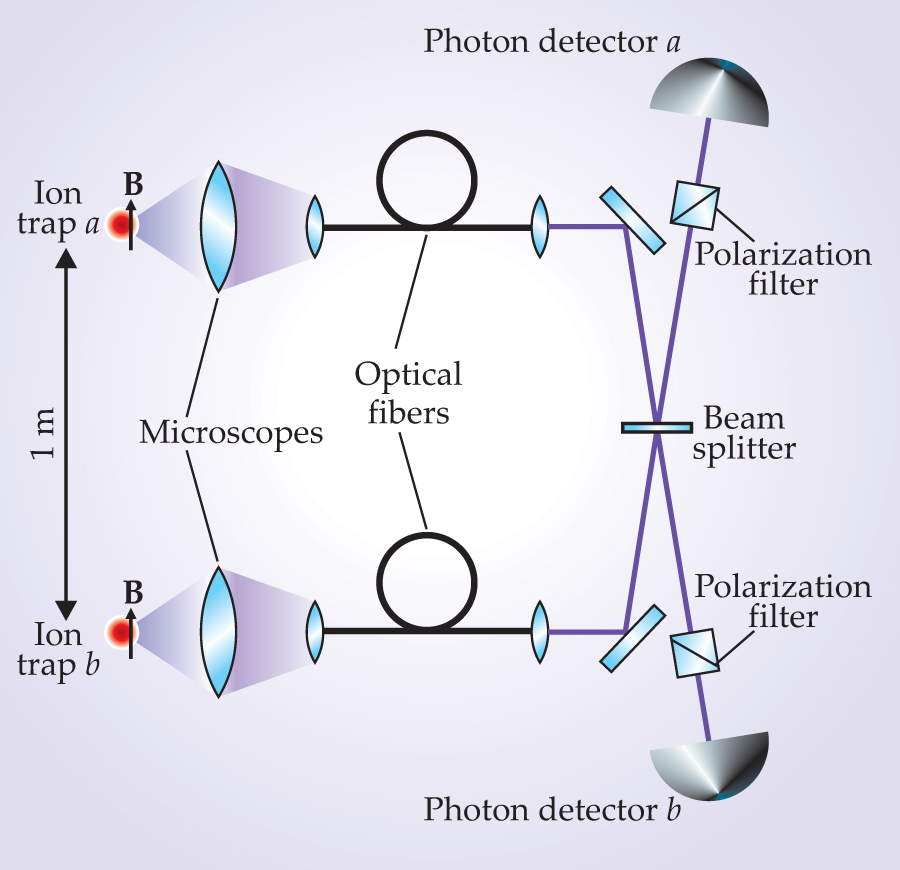
As shown schematically in figure 2, microscopes were focused at each of the ion traps to try to catch both decay photons from a given excitation pulse and direct them through optical fibers to a four-port beamsplitter and finally to two photon detectors. Along the way, polarizers blocked any photons from the decay to the |1, −1〉 S-wave state.

Before the two photons mingle at the beamsplitter’s half-silvered mirror, the only quantum entanglement is between each ion and the photon it had emitted. But then the experimenters select only those excitation events that result in photons recorded by both detectors within 15 ns after the excitation. After the photons have passed the half-silvered mirror, it’s no longer possible to say which one came from which ion. A two-detector hit heralds the existence of quantum entanglement between the hyperfine states of the two ions. Unfortunately, experimental limitations made those heralding events quite rare—about one every 10 minutes. The main reason why only a few excitation pulses per billion yield two recorded photons is the 10⁻³-steradian acceptance solid angle of each microscope.

Before the photons mingle, the joint wavefunction of hyperfine and photon states is simply a product of two wavefunctions, each describing the state of the particles from one trap. But then the requirement that both detectors record photons constitutes a measurement that collapses the wavefunction into a state in which the two ions, as well as the two photons, are entangled with each other. That comes about essentially because Bose statistics requires that if the two photons emerge from the beam splitter in opposite directions, they must be in a spin-singlet state.

The resulting joint ion wavefunction then has the entangled form

$${|\psi 〉}_{\text{ion}}=\left({|\uparrow 〉}_{\text{a}}{|\downarrow 〉}_{\text{b}}-{|\downarrow 〉}_{\text{a}}{|\uparrow 〉}_{\text{b}}\right)/\surd 2,$$ (1)

where a and b label the two traps. Its most straightforward prediction is that if one examines the two ions after both photon detectors fire simultaneously, one should always find them in different hyperfine states.

Measuring the hyperfine state

Whenever there was a simultaneous firing of both detectors, the experiment’s megahertz repetition of excitation pulses was stopped and the hyperfine states of both ions were measured by a standard fluorescence technique: Each ion was excited with a millisecond diagnostic laser pulse whose wavelength was so precisely tuned that it could excite only the |↑〉 state, raising it to the P-wave’s |0, 0〉 hyperfine substate. Once excited, the ion fluoresces as it falls back down to its original state. That cycle of excitation and decay recurs thousands of times during the millisecond laser pulse. So the diagnostic pulse unleashed a telltale bright fluorescence signal if, and only if, the ion was in the |↑〉 hyperfine state.

The experimental result for some 300 cases in which both detectors recorded photons is shown in figure 3. The two ions were found to be in different hyperfine states 78% of the time. Why not the 100% predicted by equation (1)? “It’s mostly due to electronic noise and stray radiation hitting a photon detector,” says Monroe. “The fluorescence hyperfine measurement itself is about 97% accurate.”

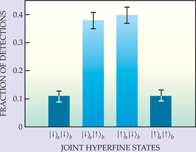
Figure 3 is only a very preliminary test of quantum entanglement. It’s like using two coordinated Stern–Gerlach analyzers always oriented alike to measure the spin projections of a pair of separated electrons entangled in a spin-0 state along the same axis. Although each measurement result appears to be random, the two electrons always yield opposite results.

Such limited correlation, by itself, is not nearly spooky enough to deserve the epithet quantum weirdness. one can, after all, imagine a classical analogue: Two prisoners about to be questioned in separate cells want to coordinate their answers to a series of yes–no questions they can’t predict. That’s easily done—even without resort to the truth—so long as both are asked the same questions in the same order. They could, for example, agree beforehand that their answers to the nth question would be determined by the parity of the nth digit in the decimal expansion of π.

But when the questions are uncorrelated as well as unpredictable, classical analogues become impossible and violations of Bell’s inequality appear. That’s effectively what the Freedman and Aspect experiments demonstrated when they confirmed the quantum mechanically predicted correlation of the polarizations of entangled photons as measured in separated, differently oriented analyzers.

Demonstrating entanglement

Instead of rotating the relative orientation of two Stern–Gerlach or polarization analyzers, Monroe and company used microwave pulses to rotate the hyperfine eigenstates in Hilbert space independently in each trap before testing the spooky correlation predicted by quantum mechanics. That’s effectively equivalent to demonstrating entanglement by independently rotating the analyzers.

Each of the 300 hyperfine measurements plotted in figure 3 was done immediately after a recording of simultaneous hits in both photon detectors—without any further tampering with the ions before their hyperfine states were measured. But most of the time after a two-detector hit, the group did tamper with the ions before measuring their hyperfine states.

Typically after a two-detector hit, each ion was subjected to a 12.6-GHz microwave pulse before the fluorescence hyperfine measurement. That frequency corresponds to the energy splitting of 6 × 10⁻⁵ eV between the |↑〉 and |↓〉 substates. The pulse’s intensity and 4 μs duration were chosen to ensure that both of those eigenstates become coherent superpositions $\left(|\uparrow 〉\pm e^{i\phi }|\downarrow 〉\right)/\surd 2,$ , where the quantum mechanical phase angle φ is determined by the phase of the microwave radiation.

What matters is the difference Δφ = φ_a - φ_b between the phases of the two trapped ions. The experimenters controlled Δφ by having the magnetic-field intensity B differ slightly between the two traps and imposing a variable time delay Δt on the irradiation of one trap relative to the other from the common microwave source. The B difference produced a part-in-10⁶ mismatch between the hyperfine splittings in the two traps. As a result, Δφ cycled in and out of phase as a function of the delay with a period of about 100 μs.

If the two ions had invariably been in the entangled state of equation (1) before microwave rotation, and if the rotations preserved their coherence perfectly, the fraction of ions found in opposite hyperfine states should simply be (1 + cosΔφ)/2. Figure 4 shows the measured fraction in opposite states, plotted as a function of Δt, which is approximately (100 μs/2π)Δφ.

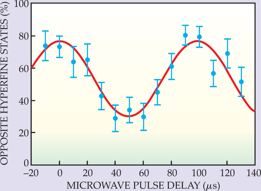
The data do exhibit the sought-after sinusoidal variation that demonstrates quantum entanglement. But, as in figure 3, the amplitude of the variation is limited by the roughly 22% admixture of events in which both ions have the same hyperfine state even before microwave rotation—mostly as a result of noise or accidental coincidences.

“The best way to increase the rate at which we see entangled events would be to hold each ion in an optical cavity,” says Monroe. “That way we’d be able to catch most of the decay photons. We’re working on it. in the meantime, we’ve already improved our entanglement rate a lot by exploiting photon polarization in a somewhat different excitation and decay scheme.”

At the end of September, Monroe and most of his coauthors—together with their equipment—moved to the Joint Quantum Institute at the University of Maryland, College Park. JQI is a joint undertaking of the university and NIST in nearby Gaithersburg, Maryland.

Entanglement underlies most schemes for quantum computing. And Monroe’s experiment was meant to show that distance is not an impediment to preserving quantum memory in atoms. “It’s a proof-of–principle demonstration of an effect that can be used to perform quantum logic operations between remote qubits and registers,” says Harvard atomic physicist Mikhail Lukin. For example, entangled atoms separated by regular intervals might serve as “quantum repeaters” to refresh the memories of photons transporting quantum information over long distances. one could have large-scale distributed quantum computing. “Monroe’s experiment,” says Lukin, “could form the basis for one of the realistic routes toward scalable quantum information systems.”

References

1. J. S. Bell, Physics 1, 195 (1964).
2. D. L. Moehring et al., Nature 449, 68 (2007). https://doi.org/10.1038/nature06118