Machine-learning-assisted modeling

To understand problems in biology, chemistry, engineering, and materials science from first principles, one can start, as Paul Dirac advocated, with quantum mechanics. ¹ Scientific advances made since the early 20th century attest to that view. But solving practical problems from a quantum mechanical perspective using the Schrödinger equation, for example, is a highly nontrivial matter because of its various complexities. To overcome the mathematical difficulties, researchers have proceeded along three lines of inquiry: looking for simplified models, finding approximate solutions using numerical algorithms, and developing multiscale models.

Each of those approaches has advantages and disadvantages. Simplified models—a constant theme in physics—capture the essence of a problem or describe some phenomenon to a satisfactory accuracy. Ideally, simplified models should have the following properties: They should express fundamental principles, such as conservation laws; obey physical constraints, such as symmetries and frame indifference; be as universally applicable as possible; be physically meaningful or interpretable; and require few externally supplied parameters.

One particularly successful simplified model is Euler’s set of equations for gas dynamics. They accurately model dense gases under general conditions and are less complex than their quantum equivalents. For ideal gases, the only parameter required is the gas constant. For complex gases, one needs the entire equation of state, which is a function of only two variables. Other success stories include the Navier–Stokes equations for viscous fluids, linear elasticity equations for small deformations of solids, and Landau’s model of phase transitions.

Unfortunately, not every effort to develop simplified models has been as successful. A good example is the work of extending Euler’s equations to rarified gases. ² Since the mid 20th century, researchers have made numerous efforts to develop Euler-like models for the dynamics of gases whose molecular mean free path exceeds the system’s relevant length scale. But so far none of those models has been widely accepted.

For systems in which analytical solutions are rare or unobtainable, one has to resort to numerical algorithms. Many such algorithms, including finite difference, finite element, and spectral methods, solve the partial differential equations that arise in physics. The widespread availability of the algorithms has changed the way scientific and engineering applications are performed. Numerical computation now influences how researchers study fluid and solid mechanics and, to a lesser extent, atmospheric science, combustion, materials science, and various other disciplines.

Algorithms are now more or less sufficient for studying low-dimensional problems. But such studies quickly become much more difficult as the dimensionality, or the effective degrees of freedom, increases beyond three. The issue that lies at the core of many difficult problems is the curse of dimensionality: As the dimensionality grows, the complexity, or computational cost, grows exponentially.

One idea to overcome modeling difficulties that can’t be ameliorated with simplified models or numeral algorithms is multiscale modeling. ³ The approach simulates the behavior of macroscale systems by using reliable models at a range of smaller scales instead of relying on ad hoc macroscale models. It uses the results of the microscale model on much smaller spatial and temporal domains to predict the macroscale quantities of interest. That general philosophy is valid for a range of scientific disciplines. But the success of multiscale modeling has been less spectacular than what was expected 20 years ago. Many factors are to blame, including the inaccuracy in the microscale models, the difficulty associated with moving from one scale to the next, and the lack of adequate data-processing techniques for analyzing the solutions of the microscale models to extract useful macroscale information.

Problems without good models

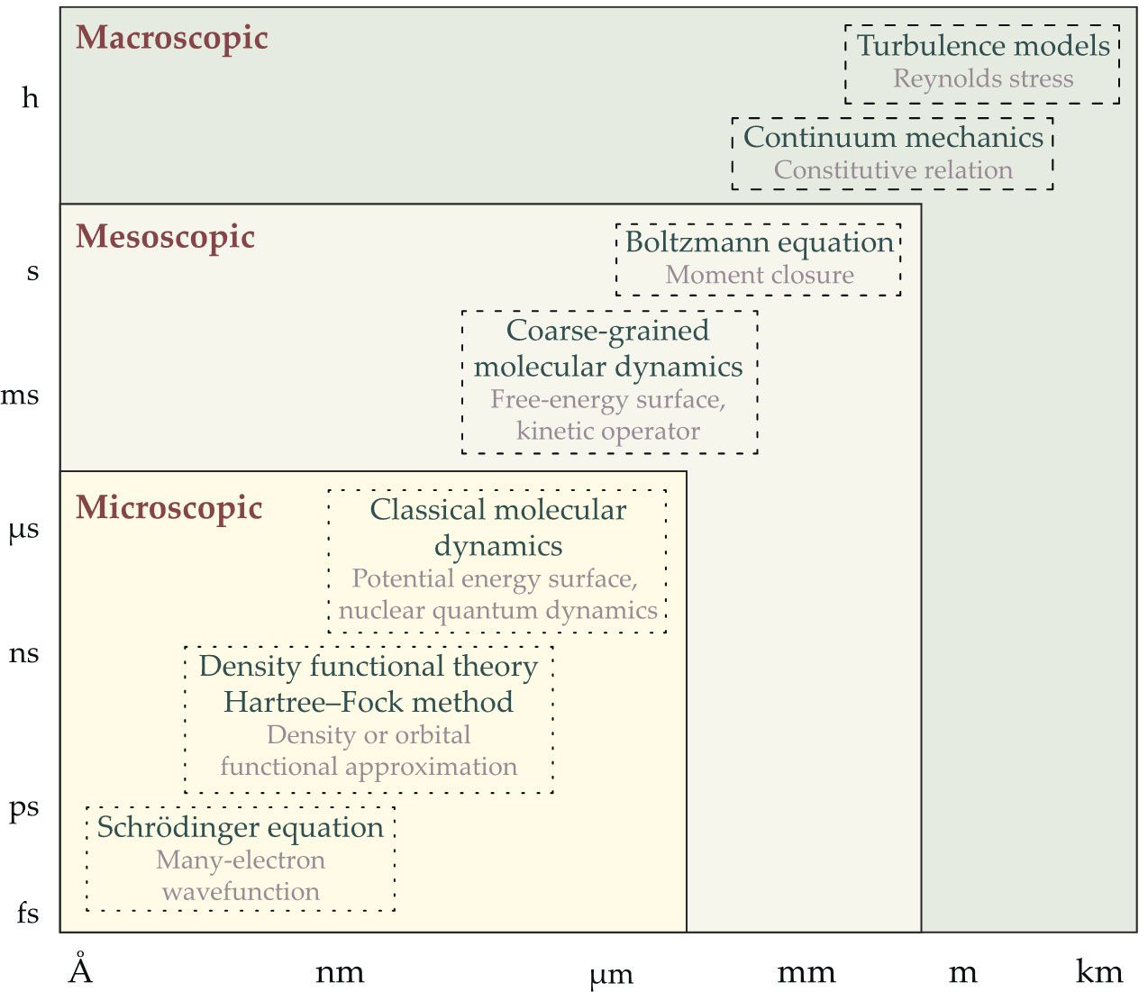
Although simplified models, numerical algorithms, and multiscale models have limitations, researchers have used them in combination with physical insight and trial-and-error fitting to solve numerous problems. Examples include performing density functional theory calculations, predicting properties of materials and molecules, and using general circulation models to study the climate. However, we still lack good models for many important areas of research, some of which are shown in figure 1.

Figure 1.

The exchange-correlation functional, for example, is a crucial component of density functional theory (see the article by Andrew Zangwill, Physics Today, July 2015, page 34 ). Formulated to embody the many-electron wavefunction, the exchange-correlation functional uses simple approximations to determine the energy associated with all exchange and correlation effects. Systematically developing efficient and accurate exchange-correlation functionals is still a challenging task. Other difficult problems include implementing coarse-grained molecular dynamics (MD) for macromolecules, developing hydrodynamic models for non-Newtonian fluids, modeling moment closure for rarified gases, and accurately representing the potential energy surface (PES) that describes the interaction between the nuclei in the system of an MD model.

The list continues. Fluids can be modeled with the Navier–Stokes equations, but what is the analogue for solids? Besides linear elasticity models, researchers hardly agree on a set of continuum models for solids, and plasticity in solids is even more problematic to simulate. Another example is turbulence models, which have faced challenges ever since the work of Osborne Reynolds in the 19th century. Physical scientists still lack the tools to systematically and robustly simulate turbulent and convective motions.

In all the identified problems, the most essential obstacle is the curse of dimensionality. Without systematic approaches, one has to resort to ad hoc procedures, which are neither efficient nor reliable. Turbulence modeling is an excellent example of the kind of pain one has to endure in order to address practical problems.

However, the problems that are made difficult by the curse of dimensionality may be more tractable because of recent advances in machine learning, which offers an unprecedented capability for approximating functions of many variables. ^{4 , 5} (See the article by Sankar Das Sarma, Dong-Ling Deng, and Lu-Ming Duan, Physics Today, March 2019, page 48 .) As spectacularly successful as machine learning is, it carries a label that is particularly harmful to applications in the physical sciences: It’s often described as functioning either as black magic or in a black box. Researchers have made substantial progress in understanding the magic behind machine learning. This article focuses on how practitioners can use machine learning to find new interpretable and truly reliable physical models. See the box on page 40 to learn more about the process that underpins neural-network-based machine learning.

Accomplishing such a task entails meeting a few requirements. First, the model should satisfy the properties listed above for ideal simplified models, although a model with only a few externally supplied parameters isn’t necessary. Second, the data set used to construct the model should represent all the practical situations the model is intended for. Fitting some data is relatively straightforward, but it is considerably more difficult to construct reliable, generalizable physical models that are accurate for all practical situations. And third, to reduce the amount of ad hoc, error-prone human intervention, the construction of the model should be automated end to end.

Concurrent machine learning

In standard approaches to supervised machine learning, researchers first provide a labeled data set to an algorithm. Then the machine-learning model interprets individual items of an unlabeled data set to, for example, recognize pedestrians in an image of a busy city street. But when machine learning is used in connection with physical models, data generation and training often become an interactive process in which data are analyzed and labeled on the fly as the model training proceeds. Analogous to multiscale modeling, ³ the standard approach can be called sequential machine learning; and the interactive process, concurrent machine learning.

For physical models derived from machine learning to be reliable, they need to be fed reliable data. The data set should ideally represent all the situations a model is intended for. For example, a reliable model for a molecule’s PES should be accurate for all the configurations that the molecule can have. But generating training data typically involves solving the underlying microscale model, which is quite often computationally expensive. Therefore, researchers usually aim to have the smallest possible data set.

To generate such data adaptively and efficiently requires a strategy such as the exploration-examination-labeling-training (EELT) algorithm. Illustrated in figure 2, it requires a macroscale explorer, a criterion to decide whether a given state or configuration should be labeled, a microscale model for labeling, and a machine-learning model for the quantities of interest. ⁶ The model is a slight modification of the exploration-labeling-training algorithm formulated in reference , though similar ideas can be traced back further. Starting without data and only a microscale model, the EELT algorithm proceeds iteratively with the following steps: (1) exploring the state or configuration space; (2) examining which configurations need to be labeled; (3) computing the microscale solutions for the states or configurations that need labeling and placing them in the training data set; and (4) training the machine-learning model.

Figure 2.

Molecular modeling

One of the most successful applications of machine learning to scientific modeling is in MD. Researchers study the properties of materials and molecules by using classical Newtonian dynamics to track the nuclei in a system. One critical issue in MD is how to model the PES that describes the interaction between the nuclei. Traditionally, modelers have dealt with the problem in several ways. One approach, ab initio MD, was developed in 1985 by Roberto Car and Michele Parrinello ⁷ and computes the interatomic forces on the fly using models based on first principles, such as density functional theory. ⁸ Although the approach accurately describes the system under consideration, it‘s computationally expensive: The maximum system size that one can handle is limited to thousands of atoms. Another approach uses empirical formulas to model a PES. The method is efficient, but guessing the right formula that can model the PES accurately enough is a difficult task, particularly for complicated systems, such as multicomponent alloys. In 2007 Jörg Behler and Parrinello introduced the idea of using neural networks to model the PES. ⁹ In that new paradigm, a quantum mechanics model generates data that are used to train a neural-network-based PES model.

To construct reliable PES models, one has to impose physical constraints and collect high-quality data. For the first problem, the main physical constraint is symmetry. In other words, the PES should be invariant under translation, rotation, and permutation of atoms of the same chemical species. As can be seen in figure 3a, even a poor man’s version of enforcing symmetry ¹⁰ can drastically improve the test accuracy. In that version, translational and rotational symmetries are enforced by fixing a local coordinate frame, and permutational symmetry is enforced by fixing an ordering of the atoms in the local coordinate frame.

Figure 3.

The only problem with the poor man’s version is that the order-fixing procedure creates small discontinuities when the ordering of the atoms near a particular atom changes. Although negligible for sampling a canonical ensemble, the discontinuities manifest themselves in a microcanonical, or constant energy, MD simulation, as shown in figure 3b. To construct a smooth PES model that satisfies all the symmetry constraints, practitioners must reconsider how to represent the general form of symmetry-preserving functions. One idea is to have the fitting network in each subnetwork succeed an embedding network that produces a sufficient number of symmetry-preserving functions and that can be optimized via training. ¹¹ In such an approach, the model automatically preserves symmetry. The idea of an embedding network can also be used in other situations in which symmetry is an important issue.

To address the second problem of generating good data, one can make use of the EELT algorithm. At the macroscale level, one samples the temperature–pressure space of thermodynamic variables. For each temperature–pressure value, the canonical ensemble is sampled using the approximate potential available at the current iteration. By adopting that procedure, only a minuscule percentage of the explored configurations need to be labeled. The constructed PES is called the deep-potential model.

Figure 4 shows the accuracy of the deep-potential model generated using the EELT algorithm. From the perspective of a materials scientist, the model achieves uniformly accurate predictions of all the target properties. ¹² When combined with the state-of-the-art, high-performance computing platform Summit at Oak Ridge National Laboratory, MD simulations with ab initio accuracy are now feasible in systems of up to 100 million atoms. The achievement makes it possible to study more complex phenomena, such as properties and dynamics of defects in materials, that require large-scale simulations ¹³ with ab initio accuracy.

Figure 4.

Moment closure in gas dynamics

The Boltzmann equation for the phase space density function of a single particle is particularly well suited for modeling the dynamics of gases. Such a simulation is rather complicated because of the dimensionality of the phase space and the complexity of the collision operator. Dense gases have long been modeled accurately using Euler’s equations, ² and since the mid 20th century, many people have tried to develop Euler-like models for rarified gases. But such modeling is difficult because of the non-equilibrium state of rarified gases.

Euler’s equations can be viewed as the projection of Boltzmann’s equation on the first few moments of the distribution function for the gas particles. Thus one possible way to develop Euler-like models for rarified gases is to generalize the moment-projection scheme by considering projections onto larger sets of moments. To get a closed model, researchers have to address terms that include moments outside of the set of moments in the projection scheme.

That issue is known as the moment-closure problem for gas dynamics. Despite many efforts and much progress over 70 years, it remains unsolved. Attempts to elucidate it are often ad hoc. Another issue is that the equations obtained may violate the second law of thermodynamics, a known issue in the 13-moment model. ²

To develop reliable and uniformly accurate Euler-like models for dense and rarified gases, researchers can use machine learning to identify not only accurate closure models but also the best set of moments to represent the distribution function. Supervised learning can find accurate closure models in much the same way as learning about a PES, as discussed earlier. Identifying the best set of moments can be solved by using an autoencoder, a well-known dimension-reduction technique in machine learning.

Another problem is that the moment-closure equations, unless corrected, violate the second law of thermodynamics. The problem is subtle and can be fixed in one of two ways. The first addresses the problem by explicitly enforcing an entropy-like condition, which is analogous to Boltzmann’s entropy-dissipation inequality. The second way sidesteps the problem by contending that as long as the model is accurate enough, it should not violate the second law of thermodynamics because the original Boltzmann’s equation does not. Therefore, our efforts should be spent on making the model uniformly accurate enough under all practical situations. Some promising results that follow the uniformly accurate approach have been obtained, ¹⁴ and a related result is shown in figure 5.

Figure 5.

The lessons learned from the moment-closure problem might be helpful in addressing other, more complex physical problems. The problem discussed in regards to gas dynamics is representative of the situation when researchers try to obtain turbulence models or hydrodynamic models for non-Newtonian fluids. In those situations, too, the closure problem needs to be addressed, and the second law of thermodynamics must not be violated.

A balancing act

Physicists are used to models based on first principles. Many of them are simple and elegant—they contain only a few parameters that are physically meaningful and measurable—and are widely applicable. Unfortunately, the world is often not so simple: Complexity is inherent to most, if not all, of the practical problems that physicists face. When dealing with complex systems, machine-learning-based models such as the ones discussed in this article may offer the solutions that researchers need.

Even though models that use machine learning are typically clumsier and involve more parameters than the ones based on first principles, they are in some ways not so different from the kinds of models we are used to. The main difference is that some functions used in the models exist in the form of subroutines. In Euler’s equations for complex gases, for example, the equation of state is stored as tables or subroutines.

In principle, the same procedure and the same set of protocols discussed in this article are also applicable in a purely data-driven context without a microscale model. In that case, the labels would be replaced with experimental results. In fact, one can imagine connecting an experimental setup to some machine-learning model using the EELT algorithm to minimize the experimental effort required for obtaining a reliable model. That promising approach remains relatively unexplored. Similar ideas are also relevant to such situations as data assimilation, in which physics- and data-driven approaches are combined to improve the overall reliability of the models. Researchers have only recently begun those kinds of efforts.

In the short term, more effort should be devoted to using machine-learning-assisted modeling to develop new reliable models for complex physical systems, such as complex fluids, and to perform optimization and control analyses on those systems. In the long term, researchers should study how to use machine learning and innovative modeling in areas such as economics, in which first-principle-based models are hard to develop.

References

1. P. A. M. Dirac, Proc. R. Soc. London A 123, 714 (1929). https://doi.org/10.1098/rspa.1929.0094
2. H. Grad, Commun. Pure Appl. Math. 2, 331 (1949). https://doi.org/10.1002/cpa.3160020403
3. W. E, Principles of Multiscale Modeling, Cambridge U. Press (2011).
4. M. I. Jordan, T. M. Mitchell, Science 349, 255 (2015). https://doi.org/10.1126/science.aaa8415
5. G. Carleo et al., Rev. Mod. Phys. 91, 045002 (2019). https://doi.org/10.1103/RevModPhys.91.045002
6. L. Zhang, H. Wang, W. E, J. Chem. Phys. 148, 124113 (2018). https://doi.org/10.1063/1.5019675
7. R. Car, M. Parrinello, Phys. Rev. Lett. 55, 2471 (1985). https://doi.org/10.1103/PhysRevLett.55.2471
8. W. Kohn, L. J. Sham, Phys. Rev. 140, A1133 (1965). https://doi.org/10.1103/PhysRev.140.A1133
9. J. Behler, M. Parrinello, Phys. Rev. Lett. 98, 146401 (2007). https://doi.org/10.1103/PhysRevLett.98.146401
10. L. Zhang et al., Phys. Rev. Lett. 120, 143001 (2018). https://doi.org/10.1103/PhysRevLett.120.143001
11. L. Zhang et al., in NIPS’18: Proceedings of the 32nd International Conference on Neural Information Processing Systems, S. Bengio et al., eds., Curran Associates (2018), p. 4441.
12. W. Jia et al., in SC’20: Proceedings of the International Conference for High Performance Computing, Networking, Storage and Analysis, IEEE Press (2020), art. 5.
13. J. Han et al., Proc. Natl. Acad. Sci. USA 116, 21983 (2019). https://doi.org/10.1073/pnas.1909854116
14. L. Zhang et al., Phys. Rev. Mater. 3, 023804 (2019). https://doi.org/10.1103/PhysRevMaterials.3.023804
More about the authors
Weinan E is a mathematics professor and Jiequn Han is a mathematics instructor in the department of mathematics and the program in applied and computational mathematics at Princeton University in New Jersey. Linfeng Zhang is a researcher at the Beijing Institute of Big Data Research in China.