Biological tissues as mechanical metamaterials
DOI: 10.1063/PT.3.4900

When a material is chosen or developed to fulfill a specific function, it transforms from an object into a tool. Concrete, for instance, is designed to support structures, whereas rubber is designed to stretch and bend. Wood is softer than steel but stiffer than nylon. Over time, scientists have amassed, through discovery and invention, naturally occurring and synthetic materials for countless applications. The ones that are chosen depend on the properties needed for the job.

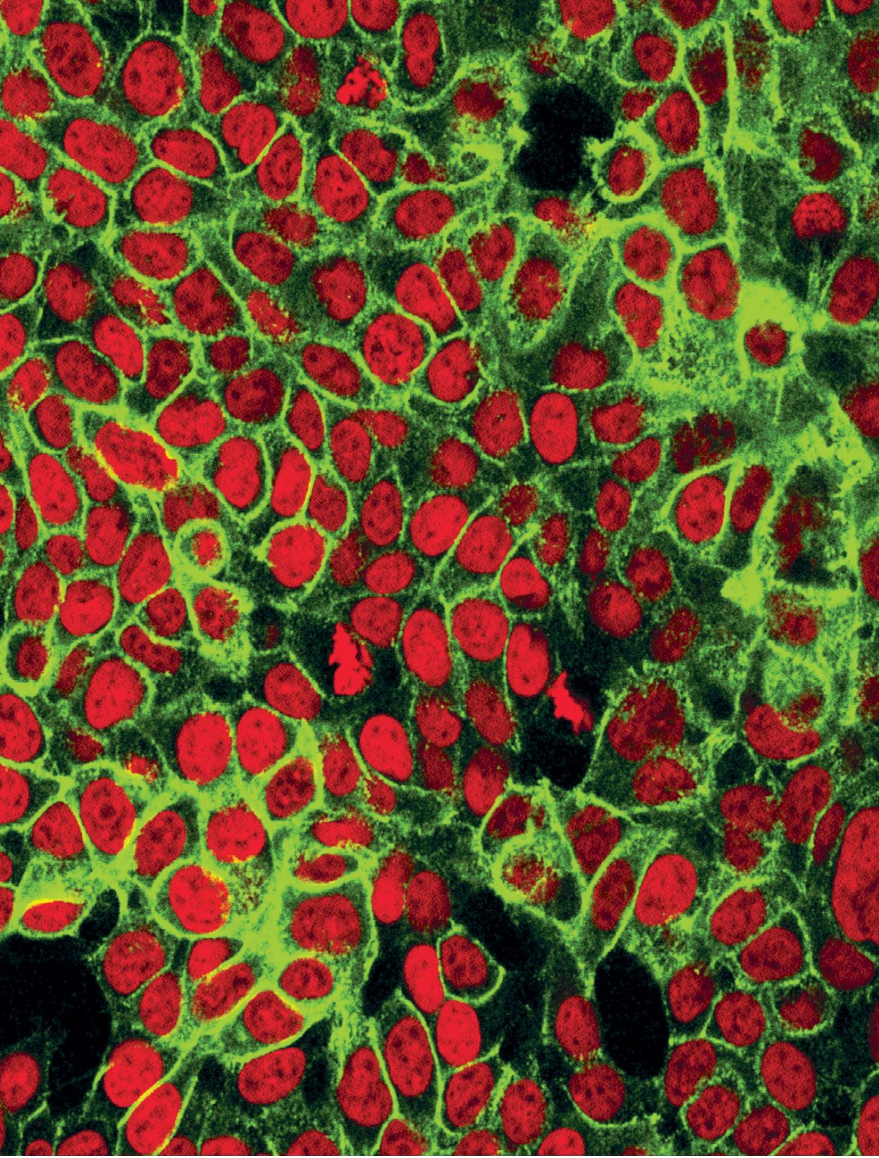
Human colon cancer cells. (Courtesy of the National Cancer Institute, National Institutes of Health.)
Materials scientists have been so successful in developing and discovering materials that researchers in the field might pause and ask ourselves what our next step is. Should we keep looking for or developing that next material, with exactly the right stiffness for some particular application? Or could we be more clever?
What if we didn’t have to pick and choose from our arsenal of materials? What if a material existed that was rigid in certain situations and flexible in others, one that changed exactly when required in order to perform specific functions? Such a material may seem like science fiction, until we realize that many biological systems are, amazingly, able to perform a multitude of tasks by dynamically adjusting their mechanical properties without changing their composition.
During an animal’s development, for example, the embryo undergoes morphogenesis, a process in which a collection of interconnected cells—a tissue—reshapes itself (see figure
Figure 1.

Epithelial cells in a Drosophila (fruit fly) embryo flow during morphogenesis. Each frame in this movie sequence, which proceeds from left to right, is separated by about 1.2 seconds. In the first two frames, the cell marked with a red dot remains roughly stationary in space, as the tissue remains solid-like. Once the tissue begins to flow, the cell moves rapidly downward, as seen in the final three frames. (Adapted from ref.
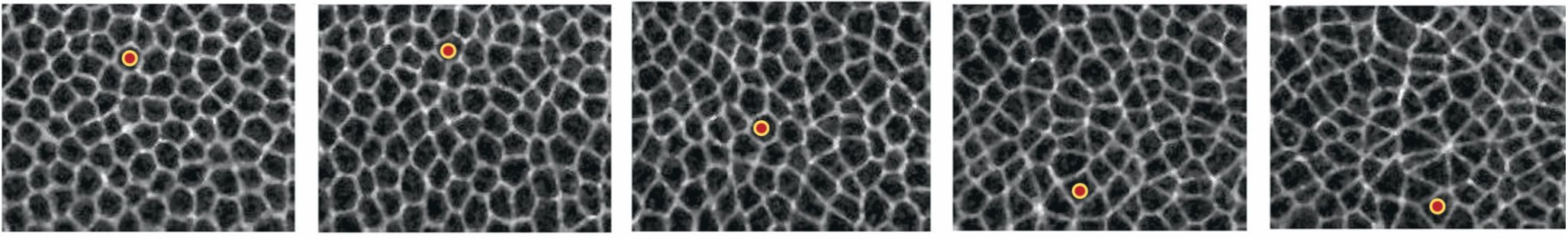
Unlike normal melting, the transformation can happen at a relatively constant temperature and is well controlled. In the morphogenesis of an embryo, the flowing tissue does not spill and spread randomly but transforms into a particular new geometry, necessary for healthy development. If materials scientists ever hope to be as clever as biology, we will first need to understand what allows such systems to function in that way. But first, we must ask a simple question: What does it mean for one material to be more rigid than another?
Constraint counting
The question of what distinguishes floppy and rigid materials turns out to be one of the oldest questions in physics, and yet it is still not easily answered. James Clerk Maxwell asked the question in the mid 1800s while thinking about macroscopic structures of rods and joints, such as truss bridges. 1
He observed that a square frame made of four rods would fall over if pushed. If one adds another rod along the frame’s diagonal, however, it prevents the frame’s collapse, as shown in figure
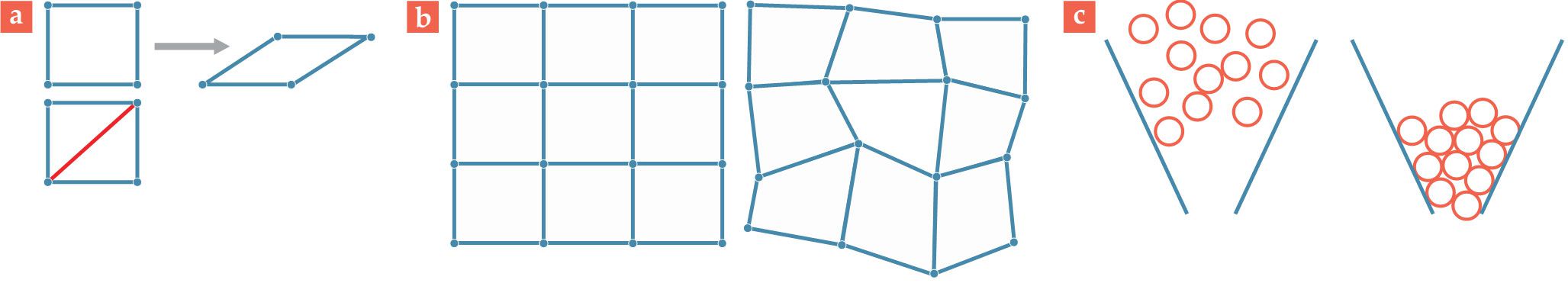
Figure 2.

Frames and forms. (a) With fewer constraints than degrees of freedom, the top frame is floppy and collapses when pushed. With an additional rod (red) on the diagonal, the bottom frame has an additional constraint, such that the structure remains rigid under pressure. (b) The crystalline solid on the left has vertices (atoms) embedded in a regular grid. The vertices in the amorphous solid on the right do not lie on a lattice. (c) The configuration of particles in the left panel allows them to flow. On the right, the particles are in a jammed, solid-like configuration.
Maxwell explained it by imagining the frame as a collection of degrees of freedom and constraints. The corners act as degrees of freedom because they can move in space, whereas the rods constrain the corners to move only in certain ways. Because any motion of a corner point can be thought of as a set of movements in each spatial dimension—forward and backward, up and down, or left and right—the total number of degrees of freedom is the number of corner points, Npts, multiplied by the number of spatial dimensions, d. Assuming that the four-rod frame can move only in the two-dimensional plane, there exist Npts × d = 4 × 2 = 8 degrees of freedom. At the same time, there are as many rods as there are points, which yields 4 as the number of constraints, Nc.
Maxwell showed that if one ignores trivial degrees of freedom, such as the translation or rotation of the entire structure, then the difference between the number of degrees of freedom (DOF) and the number of constraints reveals whether the structure is floppy or rigid. In our example, imagine that X is that difference: X = d × Npts − Nc – (trivial DOF), which becomes 2 × 4 − 4 − (2 translational + 1 rotational DOF) = 1. Because X > 0, the structure is floppy and can collapse. But once a fifth rod is added, the equation changes to X = 2 × 4 − 5 − (2 translational + 1 rotational DOF) = 0, and the structure becomes rigid. More precisely, the system is isostatic, meaning that the number of (nontrivial) degrees of freedom exactly equals the number of constraints.
If the value of X contains so much information, it must be important. But what does it represent physically? In addition to the difference between the degrees of freedom and number of constraints, its value represents the number of (again, non-trivial) ways the degrees of freedom (the corners of our frame) can be moved and yet require no mechanical energy. That is, X represents the number of zero modes—ways in which the degrees of freedom can be moved without altering the system’s energy. If any such nontrivial zero modes exist, the system is floppy. If none exist, it’s rigid.
A little more than 100 years after Maxwell published his work on the stiffness of frames, Christopher Calladine refined the method to take into account “states of self-stress”—special cases in which individual rods are tensed or compressed while the system as a whole is in mechanical equilibrium. 2 Ever since, the resulting simple, powerful Maxwell–Calladine constraint-counting method has been instrumental in mechanical engineering for building sturdy structures that can withstand external forces.
Constraint counting explains why two structures made of the same components, such as a collection of steel rods, can behave quite differently under stress. But how do we explain why steel itself is a rigid material? Remarkably, constraint counting is useful in predicting not only how rigid macroscopic structures can be but also whether microscopic structures, such as a configuration of atoms, will produce a rigid material. In fact, it turns out that the classical solid-state theory of stiffness in an atomic crystal is essentially identical to constraint counting.
In the classical picture, a solid is a collection of atoms arranged in a repeating, crystalline pattern. The structure remains cohesive because each atom interacts with its neighbors through repulsive and attractive forces. Although no rods connect atoms to each other, the interactions among the atoms act as constraints that keep them from getting too close to or too far from each other. Moreover, the interactions are usually short range, so atoms only weakly interact with other atoms that aren’t nearby. A representation of that solid—using dots to represent atoms and lines to represent constraints—looks quite similar to the macroscopic frame in the left panel of figure
Coordination number and jamming
One convenient aspect of a large system, such as a collection of atoms in a crystal, is that researchers can use statistics to analyze it. In a cubic solid, for instance, all atoms but those on the edges of the solid have six neighboring atoms; it would resemble a 3D version of figure
The number of bonds equals ½⟨z⟩ times the number of atoms Natoms in the system, where ⟨z⟩ is the average coordination number. In three dimensions the number of nontrivial degrees of freedom equals d × Natoms – 6. When the expressions are equal, the system changes from floppy to rigid. That condition thus can be used to find the value of ⟨z⟩ that sits at the transition point: ½ × ⟨z⟩ × Natoms = d × Natoms − 6, for which ⟨z⟩ = 2d – 12/Natoms. Because Natoms ≫ d in a large system, one can ignore the last term and get ⟨z⟩ = 2d.
So if the average number of neighbors is greater than or equal to twice the dimension, the system is rigid; otherwise, it’s floppy. That’s a powerful way to think about constraint counting because it means that someone can discern whether a lattice is floppy or rigid simply by knowing the number of neighbors a particle has in the lattice.
Not all materials are composed of a periodic lattice, though. Some of the most interesting and important materials, such as plastic and glass, are disordered (see the right panel of figure
That coordination-number perspective sheds light on why some systems seem to spontaneously become solid-like, without any change to their constituent particles, their temperature, or the extent to which the system of particles is disordered. Have you ever tried to pour grains of rice out of the corner of a bag? Or let coffee beans pour from a hopper at the grocery story? In both cases, the particles flow—unless they don’t. Sometimes they get stuck, transforming the system from one that behaves like a fluid to one that behaves like a solid. That jamming transition happens when the particle density increases above a critical value
4
,
5
(see figure
Mechanical metamaterials
The insights about rigidity suggest an exciting idea: One can control the mechanical properties of a system simply by controlling its geometry. That idea underlies a class of materials called mechanical metamaterials. They are manmade structures whose behavior under external forces depends on the way their components are arranged, not on their composition. Usually that kind of material relies on the geometry of a precisely constructed subunit built into the material and is the counterpart to optical metamaterials (see the article by Martin Wegener and Stefan Linden, Physics Today, October 2010, page 32 ).
By considering only its geometrical properties, researchers can design the material to behave in unusual ways, such as exhibiting auxetic behavior—when the material is compressed in one direction, it also shrinks in the perpendicular direction, as shown in the first two columns of figure
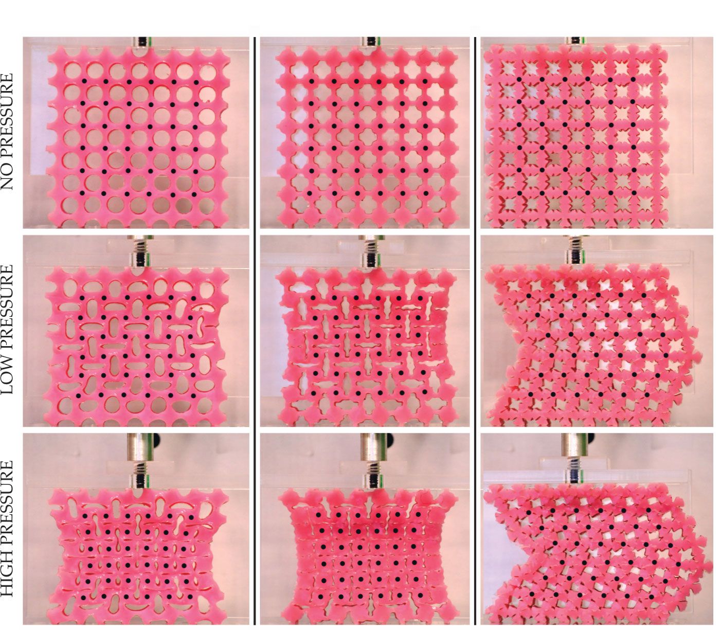
Figure 3.

Mechanical metamaterials. Three mechanical metamaterials made of the same type of rubber but with distinct geometries produce distinct behaviors under compression. Each column represents a structure, initially relaxed (top), with a unique hole shape. Whereas the hole shapes in the first two columns lead to similar behavior under compressive stress, the geometry of the holes in the last column result in a much different final configuration. The center-to-center distance between the holes is 10 mm in the relaxed configurations. (Adapted from J. T. B. Overvelde, S. Shan, K. Bertoldi, Adv. Mater. 24, 2337, 2012, doi:10.1002/adma.201104395 .)
In designing mechanical metamaterials, researchers have applied Maxwell–Calladine counting in ingenious ways. For example, some have created materials whose zero modes lie on their boundaries, where the average coordination number dips below the critical value, or come into play only when the material is deformed in a particular way. Those materials are actuatable, meaning they change their behavior rapidly upon receiving a specific (in this case, mechanical) signal. 6
Rigidity in tissues
Materials scientists have gained an understanding about the physical origin of rigidity in everything from sand piles to bridges and opened the door to a whole new class of materials. Seemingly fantastical ideas—a robotic hand, for instance, that can easily deform and flow around an object, only to quickly become rigid again to pick up the object—are now possible because of our understanding of how constituents of a material can jam. 7 To revisit the original focus of this article, it appears that we are making progress toward creating materials that act like biological tissues during the process of morphogenesis and dynamically change their mechanical properties.
But there’s a surprising catch. Look again at figure
But unlike other systems of rods or atoms, when the cellularized tissue undergoes changes to its rigidity, its number of degrees of freedom and constraints do not change. That is, none of the coordination number, temperature, or degree of disorder has to change significantly for a tissue to go from an arrested state to a flowing state.
In retrospect, the nature of the transformation is not surprising from a biological perspective. It would be inefficient and difficult for a tissue to often need to change its density—for example, via cell death or proliferation—in such a rapid and precise manner (it does happen, though; see Physics Today, June 2017, page 19 ). In fact, other biological systems, such as networks of collagen fibers, behave similarly. They do not change their connectivity but can undergo changes in stiffness. So counting degrees of freedom and constraints in those systems would not do us any good in figuring out whether they are stiff or soft. What, then, is controlling the rigidity in biological tissues and collagen networks?
Biopolymer-network models
We have more collagen in our bodies than any other protein. The collagen proteins come together to form fibers that then connect to each other to form a higher-dimensional mesh. The resulting collagen network is, in vertebrates, the primary component of the extracellular matrix (ECM), a dense composite of molecules that surrounds cells and tissues and gives them structural support.
Much like our schematics of Maxwell’s frame and an atomic solid, a schematic of the ECM also looks like a collection of rods connected at joints. The resemblance makes it again possible to count the number of degrees of freedom and constraints in the matrix in order to estimate the coordination number, or average number of connections per joint. Studies of collagen network images reveal that their average coordination number is around 3.4. That’s less than the value needed for structural rigidity in both two and three dimensions, as we saw earlier, and it means that those networks should always be expected to be floppy.
Even without changing their connectivity, however—by, say, adding, removing, or rearranging fibers—those networks can transition from weak and floppy to sturdy and rigid. In fact, that ability is biologically important, as many experiments have shown that the stiffness of the ECM acts as a signal to tissue cells. Depending on the ECM stiffness, the cells may be prompted to change or maintain their behavior. 8
To help understand the mechanical properties of such networks, researchers often use spring-network models, in which collagen fibers are represented as springs connected at points. Indeed, the rod considered in the models above can be thought of as a stiff, unbendable spring. The use of a spring allows us to explore its rodlike limit or to see what happens when connections between points are allowed to stretch or compress, much like real biological fibers. The energy it takes to compress or stretch a spring depends (quadratically) on how far away the spring length is from its preferred, or equilibrium, length.
Using such a model, researchers find that a floppy network becomes rigid when at least some of its springs are not able to reside at their preferred lengths. Importantly, that happens when the network is sufficiently strained. The network does not become more crowded, as in a jammed system, or cooler and more ordered, as in a traditional liquid-to-solid phase transition. Rather, the network experiences a geometric incompatibility. It simply cannot accommodate the newly imposed shape. 9 , 10
Vertex models of tissues
Although intriguing, the emergence of rigidity in collagen networks does not immediately seem applicable to tissues. For one thing, a tissue is a collection of cells, not interconnected fibers. Even so, if physicists are good at anything, it’s figuring out how to represent a system as a collection of springlike objects.
One such class of tissue representations is that of vertex models. They describe tissues as—you guessed it—a network of points, or vertices, connected by edges. In this case, though, the polygons created by the vertices and edges represent cells. In many vertex models, it is not the edges that have preferred lengths, as in a spring network, but the polygons (cells) that have preferred shapes.
Real cells can be surprisingly polygonal, with straight, countable sides, and tissues can sometimes even map almost exactly to a special type of vertex model called a Voronoi diagram. The locations of edges and vertices in a Voronoi diagram are determined directly from the locations of the cell centers, as shown in figure
Figure 4.

Vertex models for epithelial tissue. (a) A layer of tissue showing the cell membranes. The inset pictures a Voronoi tiling (green edges) constructed using the cell centers. The constructed edges, each consisting of points equidistant from the nearest cell centers, almost exactly match the cell boundaries. (Adapted from M. L. Zorn et al., Biochim. Biophys. Acta Mol. Cell Res. 1853, 3143, 2015, doi:10.1016/j.bbamcr.2015.05.021 .) (b) A fruit-fly wing during morphogenesis. The inset shows the cell membranes, overlaid with polygonal tiling. (Adapted from M. Merkel et al., Phys. Rev. E 95, 032401, 2017, doi:10.1103/PhysRevE.95.032401 .) (c) In this schematic of the vertex-model phase diagram, above a critical value (red dot) for the preferred cell “shape”—the ratio of the average cell perimeter to the square root of the area that the cells would like to achieve—the tissue is fluidlike, and below it is solid-like, despite no change to the tissue’s density or coordination number. (Adapted from ref.
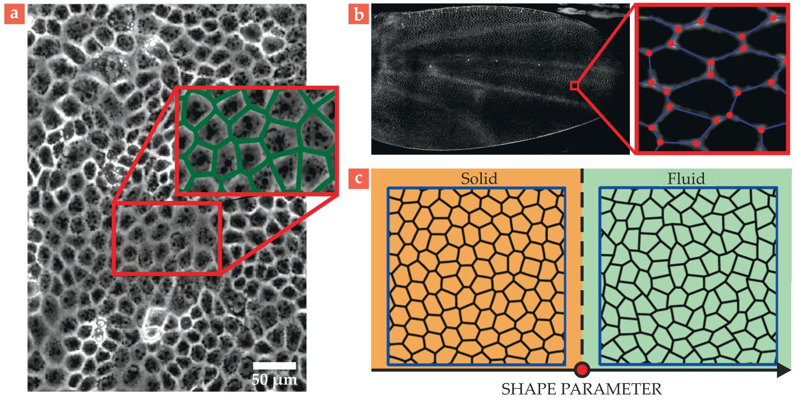
Furthermore, the idea that cells have preferred shapes comes directly from biology, which tells us that cells, being filled with water and molecules, are fairly incompressible and vary in their elasticity and affinity for sharing edges with other cells. If cells prefer contact with other cells, their edges may be long and their shapes oblong, whereas if they prefer little contact, they are more circular.
In the same way that a floppy spring network becomes rigid when its springs can no longer achieve their preferred lengths, models for confluent tissues—those with no gaps between cells—transform from flowing, fluidlike states to rigid, solidlike states when their cells can no longer achieve their preferred shapes
10–12
(see figure
Origami and the hunt for global rigidity
Researchers have now established that both collagen networks and confluent tissues have rigidities that can be tuned using parameters that represent inherent, geometric quantities—fiber length and cell shape, respectively. The process provides a way to design mechanical metamaterials with dynamic mechanical properties. It also brings us one step closer to creating materials that behave like real biological systems.
Yet an overarching question remains: Why doesn’t constraint counting work to predict rigidity in those systems? Put another way, can we know when constraint-counting arguments will work and when they won’t?
One research field that is providing clues to that mystery is the study of origami. Given a sheet of paper that can be folded only along a predetermined set of lines, how many final, folded configurations exist? Can the paper move freely from one folded state to another, analogous to the way cells in a liquid-like tissue can rearrange and flow? Or is the paper forced to take on one stable configuration, more like cells in a solidlike tissue?
It might seem useful to apply constraint counting to that system because it is composed of edges (folds) and vertices (intersections of folds). But just as in the cases of spring networks and confluent tissues, counting arguments do not correctly predict rigidity. Researchers have now discovered that the zero modes identified via constraint counting are specifically modes that do not affect the constraints to first order in a Taylor series expansion of those constraints. In some cases, however, although the first-order term in the expansion is zero, higher-order terms may not be.
In other words, because constraint counting is capable of predicting rigidity only to first order, it fails in cases where higher-order terms are important. Constraint counting turns out to be a good approximation for rigidity in some cases—which is why it seems to work for them—but in others, it’s just not good enough, and one needs to investigate how deformations of the degrees of freedom affect the constraints at higher order. 15
Mathematicians and physicists are working to figure out exactly when one can use constraint counting and when one needs to go a step further. But already, evidence is showing that the onset of rigidity in confluent tissues may be explained by using higher-order terms in an expansion of the system’s constraints. 16
What’s next?
The potential for a new material, whether biological or bioinspired, relies on understanding what truly determines structural integrity across a broad range of systems and in novel environments.
Understanding rigidity has applications in battling diseases. Cancer researchers are learning how important maintaining healthy mechanical properties of cells, tissues, and the ECM is to controlling metastasis.
17
For example, in the image on
References
1. J. C. Maxwell, London, Edinburgh, Dublin Philos. Mag. J. Sci. 27, 294 (1864). https://doi.org/10.1080/14786446408643668
2. C. R. Calladine, Int. J. Solids Struct. 14, 161 (1978). https://doi.org/10.1016/0020-7683(78)90052-5
3. H. He, M. F. Thorpe, Phys. Rev. Lett. 54, 2107 (1985). https://doi.org/10.1103/PhysRevLett.54.2107
4. A. J. Liu, S. R. Nagel, Nature 396, 21 (1998). https://doi.org/10.1038/23819
5. C. S. O’Hern et al., Phys. Rev. E 68, 011306 (2003). https://doi.org/10.1103/PhysRevE.68.011306
6. K. Bertoldi et al., Nat. Rev. Mater. 2, 17066 (2017). https://doi.org/10.1038/natrevmats.2017.66
7. E. Brown et al., Proc. Natl. Acad. Sci. USA 107, 18809 (2010). https://doi.org/10.1073/pnas.1003250107
8. J. D. Humphrey, E. R. Dufresne, M. A. Schwartz, Nat. Rev. Mol. Cell Biol. 15, 802 (2014). https://doi.org/10.1038/nrm3896
9. A. J. Licup et al., Proc. Natl. Acad. Sci. USA 112, 9573 (2015). https://doi.org/10.1073/pnas.1504258112
10. M. Merkel et al., Proc. Natl. Acad. Sci. USA 116, 6560 (2019). https://doi.org/10.1073/pnas.1815436116
11. R. Farhadifar et al., Curr. Biol. 17, 2095 (2007). https://doi.org/10.1016/j.cub.2007.11.049
12. D. Bi et al., Nat. Phys. 11, 1074 (2015). https://doi.org/10.1038/nphys3471
13. K. E. Cavanaugh et al., Dev. Cell 52, 152 (2020). https://doi.org/10.1016/j.devcel.2019.12.002
14. J.-A. Park et al., Nat. Mater. 14, 1040 (2015). https://doi.org/10.1038/nmat4357
15. B. G. Chen, C. D. Santangelo, Phys. Rev. X 8, 011034 (2018). https://doi.org/10.1103/PhysRevX.8.011034
16. L. Yan, D. Bi, Phys. Rev. X 9, 011029 (2019). https://doi.org/10.1103/PhysRevX.9.011029
17. K. R. Levental et al., Cell 139, 891 (2009). https://doi.org/10.1016/j.cell.2009.10.027
18. X. Wang et al., Proc. Natl. Acad. Sci. USA 117, 13541 (2020). https://doi.org/10.1073/pnas.1916418117
More about the authors
Amanda Parker is a computational scientist at SimBioSys in Chicago, Illinois. She is also the press ambassador for Biophysical Journal.


