Pulsed tunneling maps out an electron system’s density of states

A physical system’s otherwise hidden nature can reveal itself in the system’s response to a short, sharp, excitatory shock—which is why seismologists set off explosions in Earth’s crust and why biophysicists zap chlorophyll and its attendant proteins with laser pulses.

It’s also why MIT’s Ray Ashoori and Oliver Dial force electrons to tunnel into a thin layer of gallium arsenide millions of times a second. The electrons already in the GaAs layer adjust to each batch of newcomers. In doing so, they endow the emerging current with information about their density of states (DOS), a key quantity that experimenters measure and theorists predict.

Ashoori’s technique is a variant of two-dimensional tunneling spectroscopy. Electrons are sent tunneling at low temperature from a three-dimensional metal to a two-dimensional electron system (2DES). If the tunneling barrier preserves the electrons’ energy, the differential current dI/dV is proportional to the 2D system’s density of states.

Once they enter the 2DES, electrons thermalize within picoseconds. Using a constant DC voltage to drive the tunneling therefore risks heating the sample and distorting the DOS. To keep heating at bay, the practitioners of tunneling spectroscopy typically use low-energy electrons. In that way, they’ve found new features at and around the Fermi level (see Physics Today May 2001, page 14 ). Exploring the rest of the DOS at higher energies required a new approach.

Fourteen years ago Ashoori came up with what he calls time domain capacitance spectroscopy (TDCS): Use short voltage pulses in a capacitive AC circuit. If the pulses are short enough and the time between them long enough, repeated injections of high-energy electrons won’t heat the sample and distort the DOS.

But the briefer the pulse, the noisier the data. Figuring out how to average the millions of single measurements needed to build a clean DOS spectrum was just one of the technical challenges Ashoori and his collaborators faced.

Now, having overcome that challenge and others, Ashoori has validated his approach. He and Dial, a former grad student who stayed on as a postdoc, have mapped the DOS spectra of a quantum Hall system that occupies a semiconductor heterostructure. ¹ The spectra show Landau levels, spin splitting, and other features with a resolution and energy range that are unprecedented.

Charging up

The high-mobility heterostructure that Ashoori and Dial used in their experiment was made for them by Loren Pfeiffer and Ken West, expert crystal growers from Alcatel-Lucent’s Bell Labs. Figure 1 outlines the design.

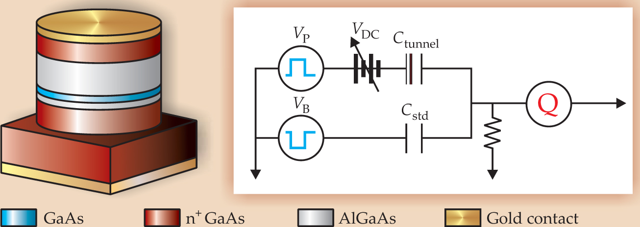
The 2D electron system (2DES) occupies a 17.5-nm thick layer of undoped GaAs sandwiched between two layers of aluminum gallium arsenide. The lower AlGaAs layer, 13 nm thick, forms the tunnel barrier. Beneath the barrier is the source of electrons, a slab of GaAs doped with so much electron-donating silicon that it’s a good conductor at low temperatures. The upper AlGaAs also abuts Si-doped GaAs, but is too thick (70 nm) to let tunneling electrons through. Gold layers at top and bottom form the electrodes.

Initially, the undoped GaAs layer is devoid of mobile, conduction-band electrons—that is, the 2DES is empty. Applying a DC gate voltage between the two electrodes draws electrons from the lower Si-doped GaAs layer through the AlGaAs tunneling barrier to populate the 2DES. The gate voltage determines the electron density, whose value can be adjusted up to 4 × 10⁻¹¹ cm⁻².

TDCS relies on applying an additional voltage, in the form of a short pulse, across the device and tracking the charge on the top electrode. Both positive and negative pulses are used, enabling the DOS to be mapped above and below the Fermi level.

Because of the capacitance between the electrodes, charge appears on the top electrode as soon as the pulse is turned on. That instantaneous—and uninteresting—charge is canceled by applying an opposite, balancing pulse to a standard capacitor in the circuit. But as electrons tunnel through the barrier, more charge arrives at the top electrode. That extra buildup, the tunneling current, embodies a piece of the DOS. How Ashoori and Dial extract those pieces and assemble the DOS is illustrated in figure 2.

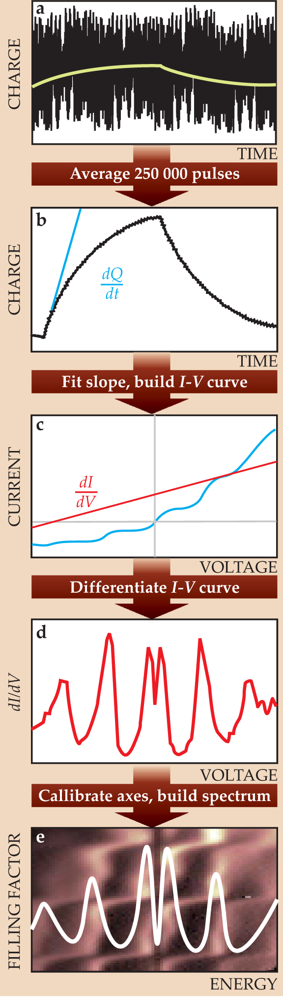
Each pulse, which lasts 50 ns and is separated from the next by 20 μs, yields a noisy, undiscernible trace of charge versus time (figure 2a). Averaging 250 000 traces reduces the noise to the required level (figure 2b).

Although figures 2a and 2b show a full trace—from the start of the pulse, through its rise, to its discharge—only the first few nanoseconds of the rise are needed to measure the tunneling current, which is given by the initial slope dQ/dt. The balancing pulse forestalls full charging.

For each value of the gate voltage, the slope is measured at 200 different values of pulse voltage. The resulting I-V curve (figure 2c) is then numerically differentiated to yield dI/dV (figure 2d). Each dI/dV curve contributes one row to the DOS spectrum. Determining dI/dV for 100 different values of the gate voltage completes a DOS spectrum.

For their proof-of-principle demonstration, Ashoori and Dial applied a strong magnetic field to drive their 2DES into the quantum Hall regime. The Landau levels that are brought into view are so distinct that they could be used to transform the axes into the more physically relevant Landau filling factor v (the number of half-filled levels below the Fermi level) and the energy of the injected or ejected electron (in meV). Figure 2e shows the final result.

The scheme’s straightforwardness belies its difficulty. Numerical differentiation entails subtracting two similar values, which reduces the signal but not the noise. The signal averaging needed to accurately determine dI/dV involved not only maintaining experimental conditions over millions of pulses but also applying sophisticated algorithms to process the signals.

Another big challenge, similar in character, arose from applying the balancing pulse. Ashoori and Dial found that the pulses from commercially available pulse generators always included a faint ringing. Subtracting two such pulses amplified the effect. Dial had to design and build his own generator. Whatever ringing it might have lay below the detection threshold of his most sensitive oscilloscope.

Figure 3 shows two DOS spectra, at 1 T and 3 T. To grasp what they show, it’s best to start with the 1 T spectrum. In general, applying a strong magnetic field perpendicular to a 2DES causes the conduction-band electrons to gyrate and forces them into Landau levels: quantized levels of energy E_n = ħΩ(n + $\raisebox{1ex}{$1$}\!\left/ \!\raisebox{-1ex}{$2$}\right.$ ), where n is a nonnegative integer and Ω = eB/m. In the 1 T spectrum, the Landau levels appear as wavy diagonal ribbons.

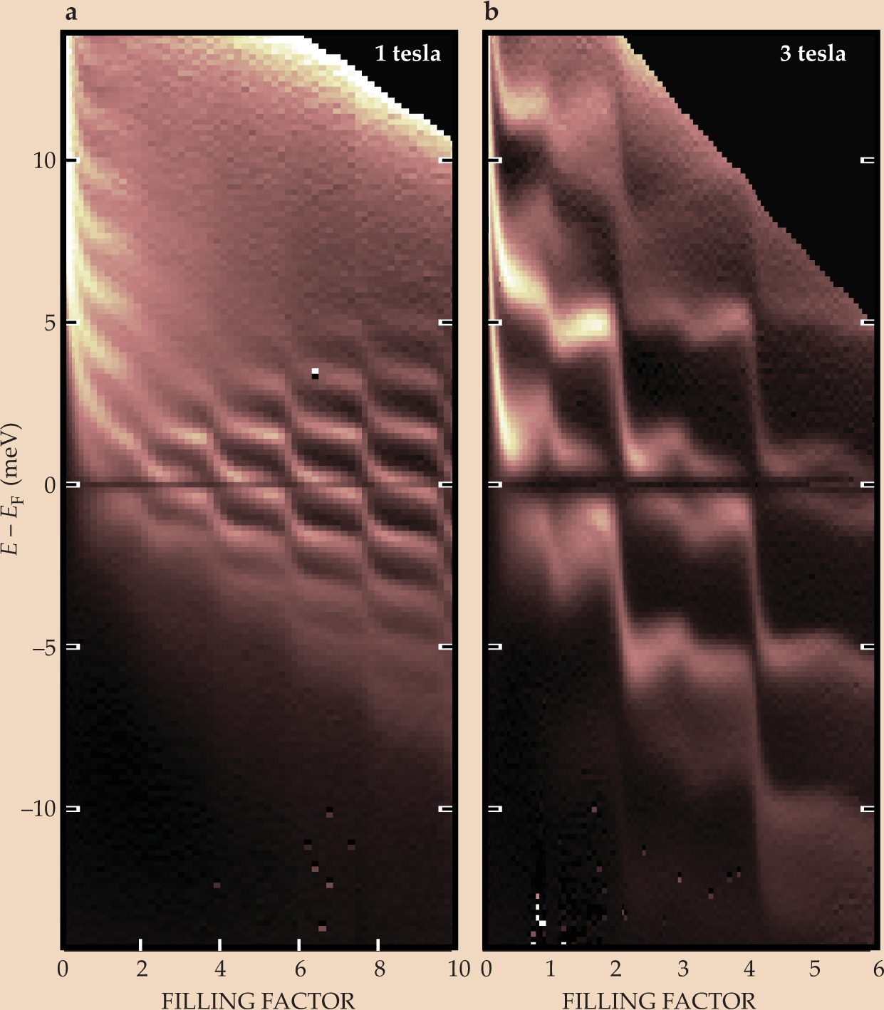
In looking at the spectrum, keep in mind that the y-axis corresponds not to the absolute value of the electron’s energy but to its excess or deficit relative to the Fermi level (y = 0). The x-axis corresponds to the gate voltage. As it’s increased, more and more electrons are added to the 2DES, which raises the Fermi level.

At zero electron density (filling factor zero), all the Landau levels appear above the Fermi level, as you’d expect for empty levels. As the density is increased, the Landau levels move down toward the Fermi level. If you follow a Landau level in the 1 T spectrum, you’ll see it flatten and get stuck when it reaches the Fermi level. It can’t sink further until it completely fills with electrons. Once full, it drops until the next level becomes pinned. Because the spectrum shows ejected and injected energy relative to the Fermi level, the Landau levels above and below the one pinned at the Fermi level also flatten.

How the electrons fill a Landau level also accounts for a prominent feature in the 3 T spectrum: the splitting at the Fermi level. Electrons in a Landau level can lower their energy by staying as far apart in their orbits as possible—which they can achieve by pointing their spins in the same direction. The energy saved by this so-called exchange splitting is highest when the maximum number of one spin species can align—that is, when a Landau level is half full. After that point, antialigned spins must be added, which reduces the size of the splitting.

Spin-based splitting also appears in the fully occupied Landau levels that lie below the Fermi level and in the completely empty levels above. There, the energy-saving alignment arises between electrons in different Landau levels, a phenomenon called indirect exchange.

The black band that runs along the Fermi energy arises from the so-called Coulomb gap. When an electron emerges from the tunneling barrier, it has to push aside electrons already present in the updoped GaAs layer. Under an applied magnetic field, those electrons, once pushed, gyrate back to their places and make it harder for the newcomer to settle in. If the newcomer arrives with little additional energy—that is, if it tunnels close the Fermi level—it’s driven back into the barrier and can’t contribute to the DOS spectrum.

The spectra’s calibration—from voltages to filling factor and energy—is secure enough to compare the data directly with theory. Ashoori and Dial measured the exchange splitting E _ex at various values of the filling factor v and magnetic field B. They found E _ex ∞ v ⁻ $\raisebox{1ex}{$1$}\!\left/ \!\raisebox{-1ex}{$2$}\right.$ B. That dependence is not predicted by theory.

Ashoori and Dial also measured the lifetime of the states occupied by the tunneling electrons. Lifetime, which corresponds to energy broadening, shows up in DOS spectra because the magnetic field pushes the electrons into narrow Landau levels. When scattering or some other process causes the electrons to lose or gain energy, the Landau levels widen.

Fermi liquid theory predicts that lifetime depends on the number of states the electron can decay into when it uses all or some of its energy to eject an electron from the Fermi sea. A low-energy electron has only enough energy to knock out electrons from the shallow top layer. A high-energy electron, by contrast, can knock out electrons from a greater range of depth. In the DOS spectra, lifetime broadening therefore increases away from the x-axis.

Disorder, in the form of impurities and lattice defects, also broadens levels through inelastic scattering. The effect of disorder can be mitigated somewhat by the presence of electrons, which screen defects and impurities. Screening increases with electron density, so lifetime broadening increases away from the y-axis.

In 1971 Alexander Chaplik derived an analytic expression for lifetime broadening. ² In the parts of the spectrum where disorder is unimportant, Chaplik’s expression provides a good fit with no free parameters.

For all its impressive range and resolution, TDCS has some limitations. The DOS depends not only on energy but also on momentum k. Angle-resolved photoemission spectroscopy can measure the k dependence, unlike TDCS and other tunneling spectroscopies. But because ARPES works by ejecting electrons and measuring their momenta, it can’t be used in applied magnetic or electric fields.

The Coulomb gap provides another limitation. As the applied magnetic field is increased, the gap widens and blots out more of the DOS—just where Ashoori and Dial have started to see new and interesting features. High fields also cause high-energy electrons to lose energy and fall into the Coulomb gap. To get them out and restore equilibrium in time for the next pulse, Ashoori and Dial apply an extra discharge pulse, whose timing and amplitude require painstaking feedback.

That the approach requires a heterostructure is also somewhat of a limitation. Not all materials are amenable to molecular beam epitaxy, the technique Pfeiffer, West, and others use to make heterostructures. Still, there are some promising candidates. Ashoori has teamed up with Ivan Bozovic at Brookhaven National Laboratory. Bozovic is making a heterostrucure out of another interesting 2DES, the high-T _c superconductor lanthanum strontium cuprate.

References

1. O. E. Dial, R. C. Ashoori, L. N. Pfeiffer, K. W. West, Nature 448, 176 (2007). https://doi.org/10.1038/nature05982
2. A. V. Chaplik, Sov. Phys. JETP 33, 997 (1971).