Experiment tracks the progress of a chaotically mixed chemical reaction

If you drop a spoonful of sour cream into a bowl of borscht, the two liquids will barely mix. But if you stir them, the spoon will drag filaments of cream through the soup. Stir further, and the filaments will stretch and fold. Eventually, if that’s your taste, the cream and soup will blend.

How stirring converts a spatially inhomogeneous state into a homogeneous one seems like the sort of problem G. I. Taylor might have solved in the 1930s. But only in the past 20 years have the mathematical tools become available to build plausible theories.

Those theories have advanced to include components that react with each other. Now, they’re being tested in the lab. Paulo Arratia of the University of Pennsylvania in Philadelphia and Jerry Gollub of Haverford College near Philadelphia have developed an experiment that tracks the progress of a chemical reaction in a stirred solution. ¹

To their surprise, Arratia and Gollub discovered they could predict the growth of chemical product under a variety of conditions by measuring a single parameter of the fluid flow. The parameter, the mean Lyapunov exponent, characterizes the rate at which fluid elements stretch and separate.

Arratia and Gollub’s experiment runs in a time-periodic regime called chaotic advection. Like turbulence, chaotic advection separates fluid elements exponentially in time, but the flow is less vigorous. Chemical engineers, who want to mix things efficiently, prefer turbulence, but for viscous liquids or small vessels, chaotic advection is sometimes the only choice.

Stirred not shaken

Flows stretch and move fluid elements, thereby increasing the opportunities for the reactants to meet and combine. To measure the stretching, Arratia and Gollub used an apparatus that Gollub developed in 2002 with Haverford’s Greg Voth and MIT’s George Haller.

In the two-dimensional setup, the fluid occupies a shallow square tray, 15 cm wide and 5 mm deep. The fluid’s velocity field is measured by imaging the changing positions of 500 microscopic latex tracers dispersed in the fluid.

To create a velocity field in the first place, one needs to shake the container or stir the fluid. Both methods create troublesome inhomogeneities at the walls of the container or at the edges of the stirrer. Voth, Haller, and Gollub solved the boundary problem by using an electromagnetic technique pioneered in the 1990s by Patrick Tabeling of the School of Industrial Physics and Chemistry in Paris.

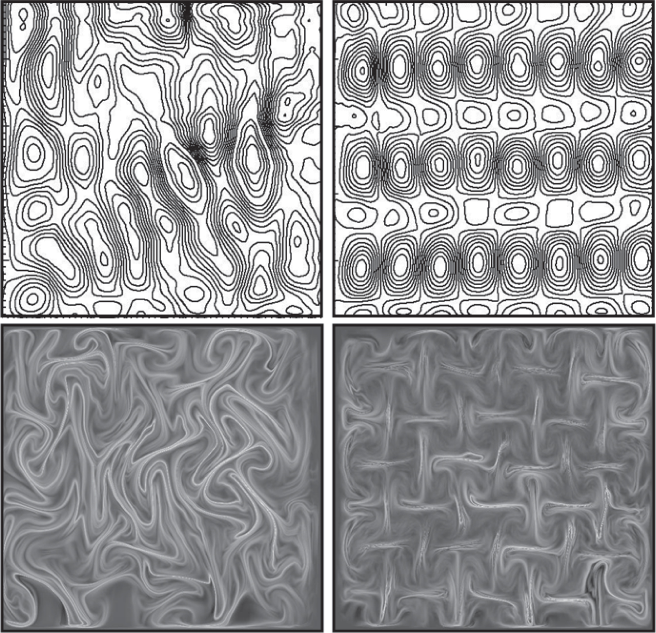
They make the fluid electrically conductive and position the tray on top of an array of 30 or so magnets. Applying a periodic electric field across the tray drives the fluid back and forth over the magnets. Lorentz forces do the stirring. Arranging the magnets in a regular or random pattern creates a more or less symmetric velocity field, as shown in figure 1.

As the fluid elements stretch and fold, the interfaces between reactants lengthen dramatically and sharpen in the direction perpendicular to the interface. The diffusion of reactants toward each other is enhanced, speeding the reaction.

Arratia and Gollub investigated the archetypical aqueous acid–base reaction HCl + NaOH → NaCl + H₂O. Because the reacting solution isn’t particularly conductive, Arratia and Gollub floated it in a thin layer on top of the stirred conducting fluid. The reaction is fast. A typical run would take a second to complete.

At the start of the experiment, the acid and base solutions were kept apart. To monitor the reaction’s progress, Arratia and Gollub added a pH-sensitive fluorescent dye to the acid. Once the barrier was removed and the electromagnetic stirring began, the local intensity of the fluorescent signal traced the change of pH as acid and base neutralized each other.

Lyapunov exponents

Mixing is more closely related to the stretching and folding of fluid elements than to their velocity. By tracking tracers in their stirred fluid, Arratia and Gollub measured the velocity field. From it, they derived the stretching field—that is, the local distortion of an infinitesimally small fluid element.

One way to characterize local stretching is through an exponent devised more than a century ago by Alexander Lyapunov. After a time Δt, two originally adjacent fluid elements separate by a distance exp(λΔt), where λ is the Lyapunov exponent. In smooth and steady flows, λ is zero throughout. In chaotic and turbulent flows, λ varies from point to point.

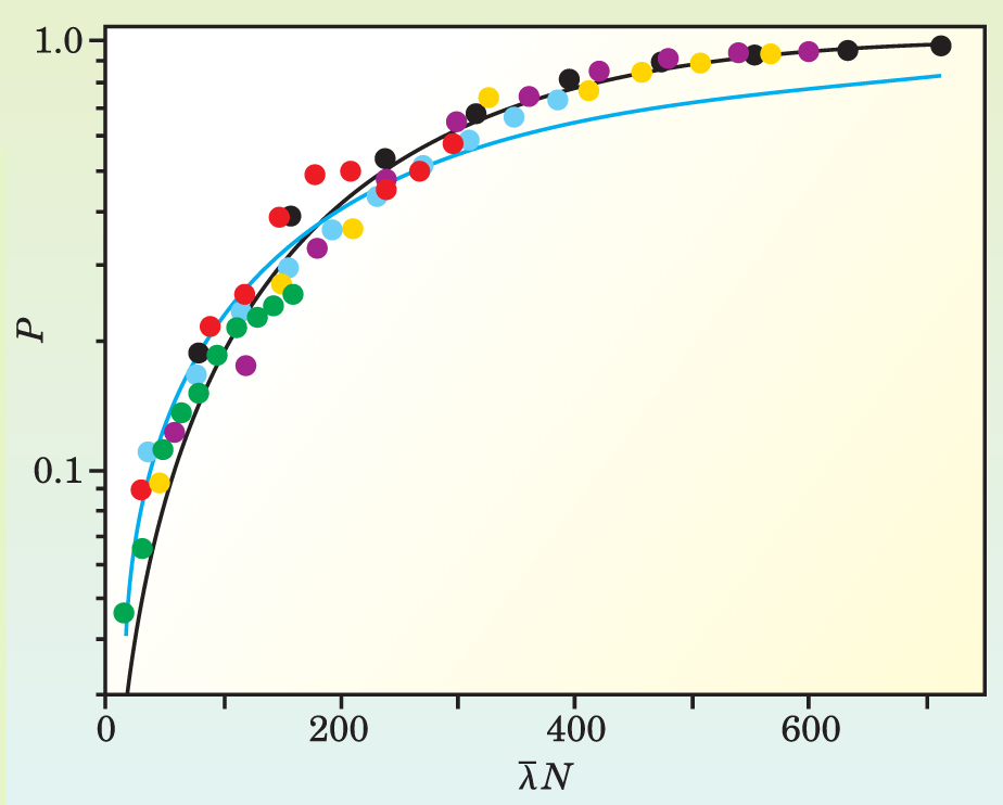
Arratia and Gollub ran their experiment for a range of Reynolds numbers and magnet arrangements. And they plotted how P, the total amount of chemical product, increased as a function of various quantities, including N, the number of times the electric field was switched back and forth, and $\overline{\lambda }$ , the average Lyapunov exponent.

As expected, P increased with both N and $\overline{\lambda }$ . Raising the Reynolds number accelerated the increase, as did arranging the magnets aperiodically rather than periodically. But fluid dynamicists, like other physicists, seek evidence of universal, predictive behavior. In the hope of finding it, Arratia and Gollub plotted P against various quantities. When they used $\overline{\lambda }$ N as the x-axis, they discovered all their curves collapsed to one. Figure 2 shows the result.

Can theory account for the figure? In a recent paper, György Károlyi of Budapest University of Technology and Economics and Támas Tél of Eötvös University, which is also in Budapest, applied the techniques of deterministic chaos to the problem. ² Their analysis, which relies on Károlyi’s concept of a time-dependent fractal dimension, predicts that P should rise as $1-exp\left(-\alpha \overline{\lambda }N\right)$ , where α is a constant. The model, represented by the blue curve in figure 2, accounts for the data at early times but fails at later times. The black curve, which has the form $1-exp\left[-\alpha \overline{\lambda }N-\beta {\left(\overline{\lambda }N\right)}^2\right]$ , fits better but is purely empirical.

Gollub notes that fluid elements, in addition to being stretched and folded, can also be transported by flows. Transport, he speculates, could be the missing ingredient that a successful physical model should contain.

References

1. P. E. Arratia, J. P. Gollub, Phys. Rev. Lett. (in press).
2. G. Károlyi, T. Tél, Phys. Rev. Lett. 95, 264501 (2005).