Analysis reveals when evolution favors one mode of gene regulation over another

Lactose isn’t present in our guts all the time. To ingest it and other occasional sources of nutrition, Escherichia coli must detect the molecules and then make the proteins that help harvest them.

That process of on-demand protein production is an example of gene regulation. Without gene regulation, an organism’s genetic code would remain an unread list of unmade proteins. Gene regulation controls when and where proteins are made and in what quantities.

Nature has evolved several modes for gene regulation, some of which involve casts of multiple molecular actors. Among the simplest are two modes used by E. coli to make the best use of randomly available sources of food. How those two modes evolved is the subject of a new analysis by physicists Ulrich Gerland of the University of Munich in Germany and Terence Hwa of the University of California, San Diego. ¹

The two modes are depicted in figure 1. In double-positive (++) control, proteins called transcription factors float freely in the bacterium’s cytoplasm. When a TF molecule encounters a lactose or other nutrient molecule, the two molecules bind. The act of binding alters the TF’s shape and enables it to latch onto the bacterium’s single strand of DNA.

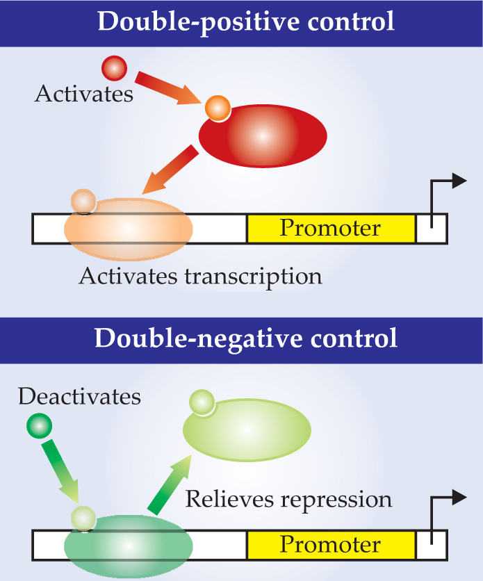
The TF binding site lies upstream of a sequence of DNA called a promoter. The promoter in turn lies upstream of the gene that encodes the TF-regulated protein. By binding to the DNA, the TF activates the promoter’s ability to attract the transcription enzyme RNA polymerase. Once RNAP is engaged, the expression of the gene into protein begins.

Double-negative control (−−) involves a similar set of molecules, but it works in the opposite way. Another kind of TF represses gene expression so long as it’s bound to DNA. When a nutrient molecule binds to it, the TF changes shape and detaches from the DNA, thereby activating the promoter, lifting the repression, and initiating transcription.

Both modes have the same effect: A gene is expressed in the presence of a nutrient molecule. Why, then, does E. coli use two modes? When does it use one mode and not the other? In a pioneering 1974 investigation, Michael Savageau correlated the modes with the concentration of various nutrients in the human colon. ² He found that (++) control is favored when a nutrient is more frequently present than not, whereas (−−) control is favored when a nutrient is more frequently absent than not.

That preference makes sense from one evolutionary perspective. Random mutations can prevent a TF molecule from binding to DNA and fulfilling its role. Therefore, Savageau argued, the more time TF spends bound to DNA, the less time is available for unbound TF to develop a function-destroying mutation. He dubbed that selection principle “use it or lose it.”

Gerland and Hwa recognized that another, opposing principle could be in play. DNA incurs random mutations all the time. Because of the genetic code’s redundancy, many mutations have no effect; they are neutral. For example, four different three-letter codons encode the simplest amino acid, glycine. Changing one letter to another could still yield glycine. But over time, the mutations accumulate and the genetic code drifts. In a small population, genetic change, good or bad, can become fixed. (For more on population genetics, see the article by Oskar Hallatschek and David Nelson on page 42 of this issue.)

The risk of genetic drift causing a TF to become dysfunctional is lowest for an infrequently used TF. Contrary to the use-it-or-lose-it principle, adverse mutation is mitigated by (++) control when a nutrient is scarce and by (−−) control when a nutrient is abundant. Gerland and Hwa dubbed the selection principle “wear and tear.”

To investigate which principle prevails under what conditions, Gerland and Hwa developed a simple mathematical model. They represented the fluctuating concentration of a nutrient by a periodic box-car function: short, widely spaced cars for scarcity; long, closely spaced cars for abundance.

Mutations can kill a functioning TF, but they can also revive a dysfunctional one. Because genes, like wristwatches and cell phones, are easier to break than fix, destructive mutations are more likely than restorative mutations—10 times more likely, Gerland and Hwa assumed.

To deal mathematically with genetic drift in a finite population, they adopted the model developed in the 1930s by R. A. Fisher and Sewall Wright and the mathematical framework developed in the early 1970s by Motoo Kimura and Tomoko Ohta.

The model yielded a quantitative picture of TF evolution. For example, under famine conditions and when the food supply fluctuates much faster than the mutation rate, neither control mode has an evolutionary edge over the other. But as the fluctuations in the scarce food supply lengthen, mutations have more time to accumulate and the wear-and-tear principle increasingly prevails: Evolution selects (++) control rather than the (−−) control of use it-or-lose-it.

The effect of finite population size emerged from the model as expected, but with a twist. Small populations are more vulnerable to adverse effects of genetic drift than large populations are. Under famine conditions and when the fluctuations are modest, (−−) control emerges as the winner and use-it-or-lose-it prevails. But at a critical population size, (−−) control loses its advantage over (++) control and wear-and-tear prevails.

Gerland and Hwa ran their model for billions of generations and found rare cases where use-it-or-lose-it is literally true: In small populations, genetic drift could destroy TF function within one nutrient fluctuation period. When that happens, TF-mediated gene regulation becomes extinct until random mutations eventually restore it.

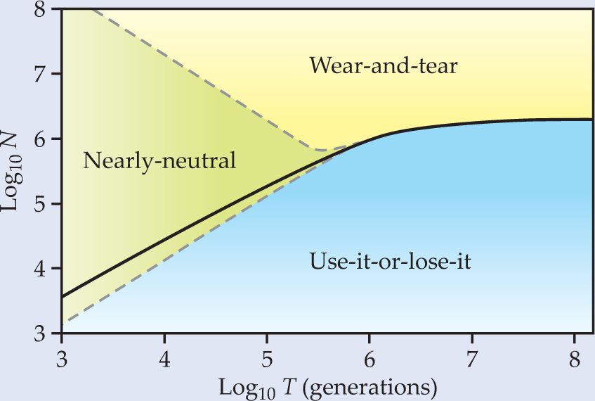
Figure 2 shows the phase diagram Gerland and Hwa derived for the case of either a hearty feast or a severe famine (the two cases are mathematically symmetrical in the model). The solid line marks the critical population at which wear-and-tear and use-it-or-lose-it are equally likely to be selected. Above the line, wear-and-tear prevails; below, use-it-or-lose-it. But how strongly a population feels that preference depends on the number of generations that have elapsed: The smaller the number, the farther a population must be from the critical line before one principle wins.

In his lab experiments, Savageau saw evidence for use-it-or-lose-it but not wear-and-tear. By applying their quantitative model, Gerland and Hwa could see why that might be the case. E. coli lives for a few hours; their mammalian hosts for a few decades. A mammal’s gut therefore hosts up to 10⁵ generations of E. coli. Given a typical colony size is also about 10⁵, Savageau’s bacteria-infected hosts were squarely in the use-it-or-lose-it region of Gerland and Hwa’s phase diagram.

Besides quantifying gene regulation, the model might help pharmacologists understand and combat the resistance of bacteria to antibiotics. One strain of E. coli, called mar, is resistant to tetracycline, an otherwise potent antibiotic, thanks to the working of two transcription factors.

References

1. U. Gerland T. Hwa, Proc. Natl. Acad. Sci. USA 106, 8841 (2009). https://doi.org/10.1073/pnas.0808500106
2. M. A. Savageau, Proc. Natl. Acad. Sci. USA 71, 2453 (1974). https://doi.org/10.1073/pnas.71.6.2453