What every physicist should know about string theory

String theory has, even among theoretical physicists, the reputation of being mathematically intimidating. But many of its essential elements can actually be described simply. This article aims to answer a few basic questions. How does string theory generalize standard quantum field theory? Why does string theory force us to unify general relativity with the other forces of nature, while standard quantum field theory makes it so difficult to incorporate general relativity? Why are there no ultraviolet divergences in string theory? And what happens to Albert Einstein’s conception of spacetime?

Anyone who has studied physics is aware that although physics—like history—does not precisely repeat itself, it does rhyme, with similar structures appearing in different areas. For example, Einstein’s gravitational waves are analogous to electromagnetic waves or to the water waves at the surface of a pond. I will begin with one of nature’s rhymes: an analogy between quantum gravity and the theory of a single particle.

Even though we do not really understand it, quantum gravity is supposed to be some sort of theory in which, at least from a macroscopic point of view, we average, in a quantum mechanical sense, over all possible spacetime geometries. (We do not know to what extent that description is valid microscopically.) The averaging is performed, in the simplest case, with a weight factor exp(iI/ℏ), where I is the Einstein–Hilbert action:

$$I=\frac{1}{16\pi G}\int d^{4}x\sqrt{g}(R-2\mathrm{\Lambda }).$$

Here G is Newton’s constant, g is the determinant of the metric tensor, R is the curvature scalar, Λ is a cosmological constant, and d⁴x is the spacetime volume element. We could add matter fields, but we do not seem to need them.

Let us try to make such a theory with one spacetime dimension instead of four. The choices for a one-manifold are quite limited:

Moreover, the curvature scalar is identically zero in one dimension, and all that’s left of the Einstein–Hilbert action is the cosmological constant. However, Einstein’s fundamental insights were not tied to the specific Einstein–Hilbert action. Rather, they were in the broader ideas that the spacetime geometry can vary dynamically and that the laws of nature are generally covariant, or invariant under arbitrary diffeomorphisms (coordinate transformations) of spacetime. (See the article by Michel Janssen and Jürgen Renn on page 30 .) By applying those insights, we can make a nontrivial quantum gravity theory in one dimension provided we include matter fields.

Adding matter

The simplest matter fields are scalar fields X_I, where I = 1, … , D. The standard general relativistic action for scalar fields is

$$I=\int dt\sqrt{g}[\frac{1}{2}\sum _{I=1}^D{g}^{tt}{\left(\frac{d{X}_I}{dt}\right)}^2-\frac{1}{2}{m}^2],$$

where g_tt is a 1 × 1 metric tensor, and the Λ term has been replaced with m²/2.

Let us introduce the canonical momentum P_I = dX_I/dt. The Einstein field equation—which is the equation of motion obtained by varying the action I with respect to g—is just

$$g^{tt}\sum _{I=1}^D{P}_I^2+m^2=0.$$

We pick the gauge g^tt = 1, so the equation is P² + m² = 0, with P² = ∑_IP_I². Quantum mechanically (in units with ℏ = 1), P_I = −i∂/∂X_I, and the meaning of the equation P² + m² = 0 is that the wavefunction Ψ(X), where X is the set of all X_I, must be annihilated by the differential operator that corresponds to P² + m²:

$$(-\sum _{I=1}^D\frac{{\mathrm{\partial }}^2}{\mathrm{\partial }{X}_I^2}+m^2)\mathrm{\Psi }(X)=0.$$

This is a familiar equation—the relativistic Klein–Gordon equation in D dimensions—but in Euclidean signature, in which time and space are on equal footing. To get a sensible physical interpretation, we should reverse the kinetic energy of one of the scalar fields X_I so that the action becomes

$$I=\int dt\sqrt{g}\{\frac{1}{2}{g}^{tt}[-{\left(\frac{d{X}_0}{dt}\right)}^2+\sum _{i=1}^{D-1}{\left(\frac{d{X}_i}{dt}\right)}^2]-\frac{1}{2}{m}^2\}.$$

Now the wavefunction obeys a Klein–Gordon equation in Lorentz signature:

$$(\frac{{\mathrm{\partial }}^2}{\mathrm{\partial }{X}_0^2}-\sum _{i=1}^{D-1}\frac{{\mathrm{\partial }}^2}{\mathrm{\partial }{X}_i^2}+m^2)\mathrm{\Psi }(X)=0.$$

So we have found an exactly soluble theory of quantum gravity in one dimension that describes a spin-0 particle of mass m propagating in D-dimensional Minkowski spacetime. Actually, we can replace Minkowski spacetime by any D-dimensional spacetime M with a Lorentz (or Euclidean) signature metric G_IJ, the action being then

$$I=\int dt\sqrt{g}(\frac{1}{2}{g}^{tt}{G}_{IJ}\frac{d{X}^I}{dt}\frac{d{X}^J}{dt}-\frac{1}{2}{m}^2).$$

From here on, summation over repeated indices is implied. The equation obeyed by the wavefunction is now the massive Klein–Gordon equation in curved spacetime M:

$$(-G^{IJ}\frac{D}{D{X}^I}\frac{D}{D{X}^J}+m^2)\mathrm{\Psi }(X)=0,$$

where D represents covariant differentiation.

Just to make things more familiar, let us go back to the case of flat spacetime (I will work in Euclidean signature to avoid having to keep track of some factors of i). Let us calculate the probability amplitude for a particle to start at one point x in spacetime and end at another point y. We do so by evaluating a Feynman path integral in our quantum gravity model. The path integral is performed over all metrics g(t) and scalar fields X_I(t) on the one-manifold

with the condition that X(t) is equal to x at one end and to y at the other.

Part of the process of evaluating the path integral in our quantum gravity model is to integrate over the metric on the one-manifold, modulo diffeomorphisms. But up to diffeomorphism, the one-manifold has only one invariant, its total length $\tau$, which we will interpret as the elapsed proper time. In our gauge g^tt = 1, a one-manifold of length $\tau$ is described by a parameter t that covers the range 0 ≤ t ≤ $\tau$. Now on the one-manifold, we have to integrate over all paths X(t) that start at x at t = 0 and end at y at t = $\tau$. That is the basic Feynman integral of quantum mechanics with the Hamiltonian being H = ½(P² + m²). According to Feynman, the result is the matrix element of exp(−$\tau$H)

$$G(x,y;\tau )=\int \frac{d^{D}p}{(2\pi {)}^D}\exp [ip\cdot (y-x)]\exp [-\frac{\tau }{2}(p^2+m^2)].$$

But we have to remember to do the gravitational part of the path integral, which in the present context means to integrate over $\tau$.

The integral over $\tau$ gives our final answer:

$$G(x,y)={\int }_0^{\mathrm{\infty }}d\tau G(x,y;\tau )=\int \frac{d^{D}p}{(2\pi {)}^D}\exp [ip\cdot (y-x)]\frac{2}{p^2+m^2}.$$

This formula is the output of the complete path integral—an integral over metrics g(t) and paths X(t) with the given endpoints, modulo diffeomorphisms—in our quantum gravity model.

The function G(x, y) is the standard Feynman propagator in Euclidean signature, apart from a convention-dependent normalization factor. Moreover, an analogous derivation in Lorentz signature (for both the spacetime M and the particle world line) gives the correct Lorentz-signature Feynman propagator.

So we have interpreted a free particle in D-dimensional spacetime in terms of 1D quantum gravity. How can we include interactions? There is actually a perfectly natural way. There are not a lot of smooth one-manifolds, but there is a large supply of singular one-manifolds in the form of graphs, such as the one in figure 1. Our quantum-gravity action makes sense on such a graph. We simply take the same action that we used before, summed over all the line segments that make up the graph.

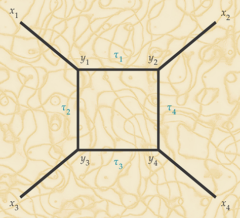
Now to do the quantum-gravity path integral, we have to integrate over all metrics on the graph, up to diffeomorphism. The only invariants are the total lengths or proper times of each of the segments. Some of the lines in figure 1 have been labeled by length or proper-time variables ${\tau }_{\mathrm{i}}$.

The natural amplitude to compute is one in which we hold fixed the positions x₁, … , x₄ of the graph’s four external particles and integrate over all the ${\tau }_{\mathrm{i}}$ and over the paths the particles follow on the line segments. To evaluate such an integral, it is convenient to first perform a computation in which we hold fixed the positions y₁, … , y₄ of the vertices in the graph. That means all endpoints of all segments are labeled. The computation that we have to perform on each segment is the same as before and gives the Feynman propagator. The final integration over y₁, … , y₄ imposes momentum conservation at each vertex. Thus we arrive at Feynman’s recipe for computing the amplitude associated with a Feynman graph—a Feynman propagator for each line and an integration over all momenta subject to momentum conservation.

A more perfect rhyme

We have arrived at one of nature’s rhymes. If we imitate in one dimension what we would expect to do in four dimensions to describe quantum gravity, we end up with something that is certainly important in physics—namely, ordinary quantum field theory in a possibly curved spacetime. In our example in figure 1, the ordinary quantum field theory is scalar ϕ³ theory because of the particular matter system we started with and because our graph had cubic vertices. Quartic vertices, for instance, would give ϕ⁴ theory, and a different matter system would give fields of different spins. Many or maybe all quantum field theories in D dimensions can be derived in that sense from quantum gravity in one dimension.

There is actually a much more perfect rhyme if we repeat the procedure in two dimensions—that is, for a string instead of a particle. We immediately run into the fact that a two-manifold Σ can be curved:

On a related note, 2D metrics are not all locally equivalent under diffeomorphisms. A 2D metric in general is a 2 × 2 symmetric matrix constructed from three functions:

$$g_{ab}=\left(\begin{array}{cc}{g}_{11}& g_{12}\\ g_{21}& g_{22}\end{array}\right),g_{21}=g_{12}.$$

A transformation of the 2D coordinates σ, generated by

$${\sigma }^a\to {\sigma }^a+h^a(\sigma ),a=1,2,$$

can remove only two functions, leaving the curvature scalar as an invariant.

All those complications suggest that the integral over 2D metrics will not much resemble what we found in the 1D case. But now we notice the following. The natural anolog of the action that we used in one dimension is the general relativistic action for scalar fields in two dimensions, namely

$$I=\int d^2\sigma \sqrt{g}{g}^{ab}{G}_{IJ}\frac{\mathrm{\partial }{X}^I}{\mathrm{\partial }{\sigma }^a}\frac{\mathrm{\partial }{X}^J}{\mathrm{\partial }{\sigma }^b}.$$

But this is conformally invariant, that is, it is invariant under a Weyl transformation of the metric g_ab → e^ϕg_ab for any real function ϕ on Σ. This is true only in two dimensions (and only if there is no cosmological constant, so we omit that term in going to two dimensions). Requiring Weyl invariance as well as diffeomorphism invariance is enough to make any metric g_ab on Σ locally trivial (locally equivalent to δ_ab), similar to what we said for one-manifolds.

Some very pretty 19th-century mathematics now comes into play. A two-manifold whose metric is given up to a Weyl transformation is called a Riemann surface. As in the 1D case, a Riemann surface can be characterized up to diffeomorphism by finitely many parameters. There are two big differences: The parameters are now complex rather than real, and their range is restricted in a way that leaves no room for an ultraviolet divergence. I will return to that last point later.

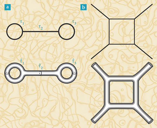
But first, let us take a look at the relation between the 1D parameters and the 2D ones. A metric on the Feynman graph in figure 2a depends, up to diffeomorphism, on three real lengths or proper-time parameters ${\tau }_1$, ${\tau }_2$, and ${\tau }_3$. If the graph is “thickened” into a two-manifold, as suggested by the figure, then a metric on that two-manifold depends, up to diffeomorphism and Weyl transformation, on three complex parameters $\tau {̂}_1$, $\tau {̂}_2$, and $\tau {̂}_3$. Figure 2b gives another illustration of the relation between a Feynman graph and a corresponding Riemann surface.

We used 1D quantum gravity to describe quantum field theory in a possibly curved spacetime but not to describe quantum gravity in spacetime. The reason that we did not get quantum gravity in spacetime is that there is no correspondence between operators and states in quantum mechanics. We considered the 1D quantum mechanics with action

$$I=\int dt\sqrt{g}(\frac{1}{2}{g}^{tt}{G}_{IJ}\frac{d{X}^I}{dt}\frac{d{X}^J}{dt}-\frac{1}{2}{m}^2).$$

What turned out to be the external states in a Feynman diagram were just the states in that quantum mechanics. But a deformation of the spacetime metric is represented not by a state but by an operator. When we make a change δG_IJ in the spacetime metric G_IJ, the action changes by $I\to I+\int dt\sqrt{g}\mathrm{𝒪}$, where $\mathrm{𝒪}$ = ½g^ttδG_IJ∂_tX^I∂_tX^J is the operator that encodes a change in the spacetime metric. Technically, to compute the effect of the perturbation, we include in the path integral a factor $\delta I=\int dt\sqrt{g}\mathrm{𝒪}$, integrating over the position at which the operator $\mathrm{𝒪}$ is inserted.

A state would appear at the end of an external line in the Feynman graph. But an operator $\mathrm{𝒪}$ such as the one describing a perturbation in the spacetime metric appears at an interior point in the graph, as shown in figure 3a. Since states enter at ends of external lines and operators are inserted at internal points, there is in general no simple relation between operators and states.

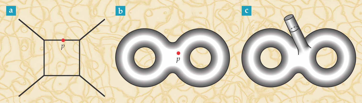
But in conformal field theory, there is a correspondence between states and operators. The operator $\mathrm{𝒪}$ = ½g^abδG_IJ∂_aX^I∂_bX^J that represents a fluctuation in the spacetime metric automatically represents a state in the quantum mechanics. That is why the theory describes quantum gravity in spacetime.

The operator–state correspondence arises from a 19th-century relation between two pictures that are conformally equivalent. Figure 3b shows a two-manifold Σ with a marked point p at which an operator $\mathrm{𝒪}$ is inserted. In figure 3c, the point p has been removed from Σ, and a Weyl transformation of the metric of Σ has converted what used to be a small neighborhood of the point p to a semi-infinite tube. The tube is analogous to an external line of a Feynman graph, and what would be inserted at the end of it is a quantum string state. The relation between the two pictures is the correspondence between operators and states.

To understand the Weyl transformation between the two pictures, consider the metric of the plane (figure 4) in polar coordinates:

$$d{s}^2=d{r}^2+r^{2}d{\theta }^2.$$

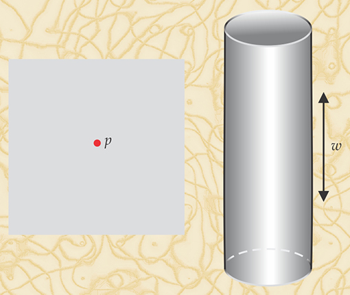
We think of inserting an operator at the point r = 0. Now remove the point and make a Weyl transformation by multiplying ds² with 1/r² to get a new metric

$$(d{s}^{\prime }{)}^2=\frac{1}{r^2}d{r}^2+d{\varphi }^2.$$

In terms of w = log r, −∞ < w < ∞, the new metric is

$$(d{s}^{\prime }{)}^2=d{w}^2+d{\varphi }^2,$$

which describes a cylinder. The point r = 0 in one description corresponds in the other description to the w → −∞ end of the cylinder. What is interpreted in one description as an operator inserted at r = 0 is interpreted in the other description as a quantum state flowing in from w = −∞.

Thus string theory describes quantum gravity in spacetime. But it does not describe quantum gravity only. It describes quantum gravity unified with various particles and forces in spacetime. The other particles and forces correspond to other operators in the conformal field theory of the string—apart from the operator $\mathrm{𝒪}$ that is related to a fluctuation in the spacetime geometry—or equivalently to other quantum states of the string.

The operator–state correspondence that leads to string theory describing quantum gravity in spacetime is also important in some areas of statistical mechanics and condensed-matter physics. That is indeed another one of nature’s rhymes.

No ultraviolet divergences

The next step is to explain why this type of theory does not have ultraviolet divergences, in sharp contrast to what happens if we simply apply textbook recipes of quantization to the Einstein–Hilbert action for gravity. When we use those recipes, we encounter intractable ultraviolet divergences that were first found in the 1930s. Back then it was not entirely clear that the problem is special to gravity, because there were also troublesome ultraviolet divergences when other particle forces were studied in the framework of relativistic quantum theory. However, as ultraviolet divergences were overcome for the other forces—most completely with the emergence of the standard model of particle physics in the 1970s—it became clear that the problems for gravity are serious.

To understand why there are no ultraviolet divergences in string theory, we should begin by asking how ultraviolet divergences arise in ordinary quantum field theory. They arise when all the proper-time variables in a loop go simultaneously to zero. So in the example of figure 1, there can be an ultraviolet divergence when ${\tau }_1$, ${\tau }_2$, ${\tau }_3$, and ${\tau }_4$ simultaneously vanish.

It is true that a Riemann surface can be characterized by complex parameters that roughly parallel the proper-time parameters of a Feynman graph (figure 2). But one important difference prevents ultraviolet divergences in string theory. The proper-time variables ${\tau }_{\mathrm{i}}$ of a Feynman graph cover the whole range 0 ≤ ${\tau }_{\mathrm{i}}$ ≤ ∞. By contrast, the corresponding Riemann surface parameters $\tau {̂}_{\mathrm{i}}$ are bounded away from zero. Given a Feynman diagram, one can make a corresponding Riemann surface, but only if the magnitudes of the proper-time variables $\tau {̂}_{\mathrm{i}}$ are not too small. The region of the parameter space where ultraviolet divergences occur in field theory simply has no counterpart in string theory.

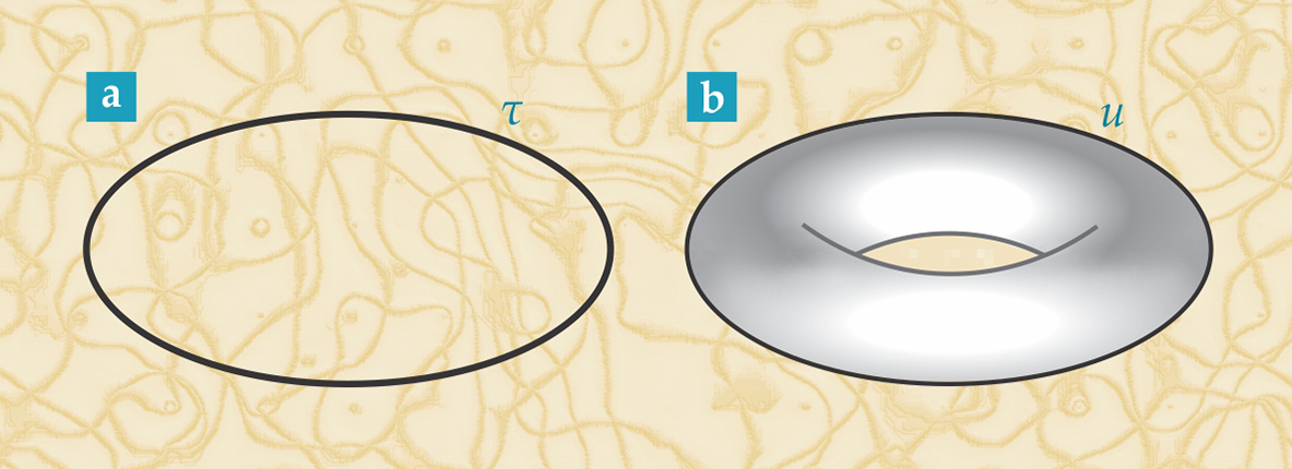
Instead of giving a general explanation, I will show how it works in the case of the one-loop cosmological constant. The Feynman diagram is a simple circle (figure 5a), with a single proper-time parameter $\tau$. The resulting expression for the one-loop cosmological constant is

$${\mathrm{\Lambda }}_1=\frac{1}{2}{\int }_0^{\mathrm{\infty }}\frac{d\tau }{\tau }Tr\exp (-\tau H),$$

where H is the particle Hamiltonian ½(P² + m²). The integral diverges at $\tau$ = 0, and the divergence is actually more severe than it looks because of the momentum integration that is part of the trace.

Going to string theory means replacing the classical one-loop diagram with its stringy counterpart, which is a torus (figure 5b). Nineteenth-century mathematicians showed that every torus is conformally equivalent to a parallelogram in the plane with opposite sides identified:

But to explain the idea without any extraneous technicalities, we will consider, instead of parallelograms, only rectangles:

We label the height and base of the rectangle as s and s′, respectively.

Only the ratio u = s’/s is conformally invariant. Also, since what we call the “height” as opposed to the “base” of a rectangle is arbitrary, we are free to exchange s and s′, which corresponds to u ↔ 1/u. So we can restrict ourselves to s′ ≥ s, and thus the range of u is 1 ≤ u < ∞.

The proper-time parameter $\tau$ of the particle corresponds to u in string theory, with the key difference being that for the particle, 0 ≤ $\tau$ < ∞, but for the string, 1 ≤ u < ∞. So in the approximation of considering only rectangles and not parallelograms, the one-loop cosmological constant in string theory is

$${\mathrm{\Lambda }}_1=\frac{1}{2}{\int }_1^{\mathrm{\infty }}\frac{du}{u}Tr\exp (-uH).$$

There is no ultraviolet divergence, because the lower limit on the integral is 1 instead of 0. A more complete analysis with parallelograms shifts the lower bound on u from 1 to $\sqrt{3}/2$.

I have described a special case, but the conclusion is general. The stringy formulas generalize the field theory formulas, but without the region that can give ultraviolet divergences in field theory. The infrared region ($\tau$ → ∞ or u → ∞) lines up properly between field theory and string theory, and that is why a string theory can imitate field theory in its predictions for behavior at low energies or long times and distances.

Emergent spacetime

My final goal here is to explain, at least partly, in what sense spacetime emerges from something deeper if string theory is correct. Let us focus on the following fact. The spacetime M with its metric tensor G_IJ(X) was encoded as the data that enabled us to define one particular 2D conformal field theory. That is the only way that spacetime entered the story.

In our construction, we could have used a different 2D conformal field theory (subject to a few general rules that I will omit for the sake of brevity). Now if G_IJ(X) is slowly varying (the radius of curvature is everywhere large), the Lagrangian by which we described the 2D conformal field theory is weakly coupled and useful. In that case, string theory matches the ordinary physics that we are familiar with. In this situation, we may say that the theory has a semiclassical interpretation in terms of strings in spacetime—and it will reduce at low energies to an interpretation in terms of particles and fields in spacetime.

When we get away from a semiclassical, weak-coupling limit, the Lagrangian is not so useful and the theory does not have any particular interpretation in terms of strings in spacetime. The potential breakdown of a simple spacetime interpretation has many nonclassical consequences, such as the ability to make continuous transitions from one spacetime manifold to another, or the fact that certain types of singularities (but not black hole singularities) in classical general relativity turn out to represent perfectly smooth and harmless situations in string theory. An example of the nonclassical behavior of string theory is sketched in figure 6.

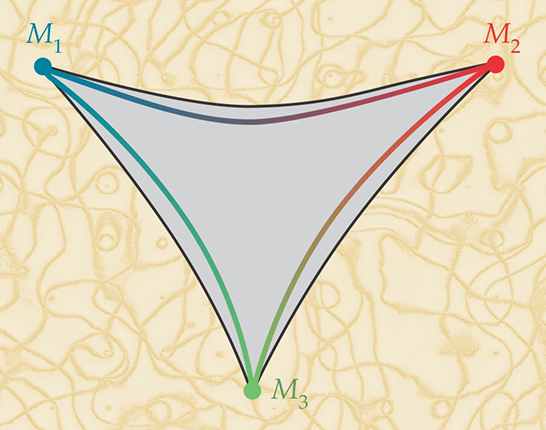
In general, a string theory comes with no particular spacetime interpretation, but such an interpretation can emerge in a suitable limit, somewhat as classical mechanics sometimes arises as a limit of quantum mechanics. From this point of view, spacetime emerges from a seemingly more fundamental concept of 2D conformal field theory.

I have not given a complete explanation of the sense in which, in the context of string theory, spacetime emerges from something deeper. A completely different side of the story, beyond the scope of the present article, involves quantum mechanics and the duality between gauge theory and gravity. (See the article by Igor Klebanov and Juan Maldacena, Physics Today, January 2009, page 28 .) However, what I have described is certainly one important and relatively well-understood piece of the puzzle. It is at least a partial insight about how spacetime as conceived by Einstein can emerge from something deeper, and thus hopefully is of interest in the present centennial year of general relativity.

References

1. B. Zwiebach, A First Course in String Theory, 2nd ed., Cambridge U. Press (2009).
2. J. Polchinski, String Theory, Volume 1: An Introduction to the Bosonic String, Cambridge U. Press (2005).
3. M. B. Green, J. S. Schwarz, E. Witten, Superstring Theory, Volume 1: Introduction, Cambridge U. Press (1987).
More about the authors
Edward Witten is the Charles Simonyi Professor of mathematical physics at the Institute for Advanced Study in Princeton, New Jersey.