Were Fundamental Constants Different in the Past?
DOI: 10.1063/1.1825267
Are any of nature’s fundamental parameters truly constant? If not, are they fixed by the vacuum state of the universe, or do they vary slowly in time even today? To fully answer those questions requires either an unambiguous experimental detection of a change in a fundamental quantity or a significantly deeper understanding of the underlying physics represented by those parameters.
At first glance, a long list of quantities usually assumed to be constant could potentially vary: Newton’s constant G N, Boltzmann’s constant k B, the charge of the electron e, the electric permittivity ∊0 and magnetic permeability µ 0, the speed of light c, Planck’s constant ℏ, Fermi’s constant G F, the fine-structure constant α = e 2/ℏc and other gauge coupling constants, Yukawa coupling constants that fix the masses of quarks and leptons, and so on. One must, however, distinguish what may be called a fundamental dimensionless parameter of the theory from a fundamental unit. Dimensionless parameters include gauge couplings and quantities that, like the ratio of the proton to electron mass, are combinations of dimensioned quantities whose units cancel. Their variations represent fundamental and observable effects.
In contrast, variations in dimensioned quantities are not unambiguously observable. (For an interesting and thought-provoking discussion on the number of fundamental units in physics, see reference .) To point out the ambiguity is not to imply that a universe with, say, a variable speed of light is equivalent to one in which the speed of light is fixed. But no observable difference between those two universes can be uniquely ascribed to the variation in c. It thus becomes operationally meaningless to talk about measuring the variation in the speed of light or whether a variation in α is due to a variation in c or ℏ. It is simply a variation in α.
Lev Okun provides a nice example, based on the hydrogen atom, that illustrates the inability to detect the variation in c despite the physical changes such a variation would cause. 2 Lowering the value of c lowers the rest-mass energy of an electron, E e = m e c 2. When 2E e becomes smaller than the binding energy of the electron to the proton in a hydrogen atom, E b = m e e 4/2ℏ 2, it becomes energetically favorable for the proton to decay to a hydrogen atom and a positron. Clearly, that’s an observable effect providing evidence that some constant of nature has changed. However, the quantity that determines whether the above decay occurs is the ratio E b/2E e = e 4/4ℏ 2 c 2 = α 2/4. Therefore, one cannot say which constant among e, ℏ, and c is changing, only that the dimensionless α is.
A brief history of time variation
The notion of time-varying constants goes back to the late 1930s, when Paul Dirac proposed his large-number hypothesis. Dirac noticed that the ratio of the electromagnetic to the gravitational interaction between a proton and an electron, e 2/G N m p m e ~ 1040, is roughly the same as the ratio of the size of the observable universe to the classical radius of the electron, m e c 3/e 2 H 0 ~ 1040, where H 0 = 70 km/(s·megaparsec) is the present-day Hubble parameter. Furthermore, both ratios are roughly the square root of the total number of baryons in the observable universe, c 3/m p G N H 0 ~ 1080. Dirac supposed that if the relationships among those ratios is not coincidence, then they should remain constant over time. Noting that the Hubble parameter is not constant (roughly speaking, it is inversely proportional to the age of the universe t), he proposed that G N ∝ 1/t. He could, however, have just as easily suggested that e 4/(m e)2 ∝ t, and the relationships among the large numbers would be maintained. Dirac’s choice naturally sets e, c, and m e as constants. However, one may rather choose Planck units, in which G N, c, and ℏ are fixed, because only the dimensionless ratios are observable.
Of course, the large-number hypothesis has been excluded by experiment. The corollary prediction (with appropriate parameters taken as fixed) that (1/G N)dG N/dt is about – 10−10/yr is some two orders of magnitude larger than the limits obtained with the Viking Landers on Mars. The limit from Big Bang nucleosynthesis is comparable.
Extensions of Albert Einstein’s theory of general relativity can realize variations in Newton’s constant. In the simplest such extension, one adds a scalar field, as described in
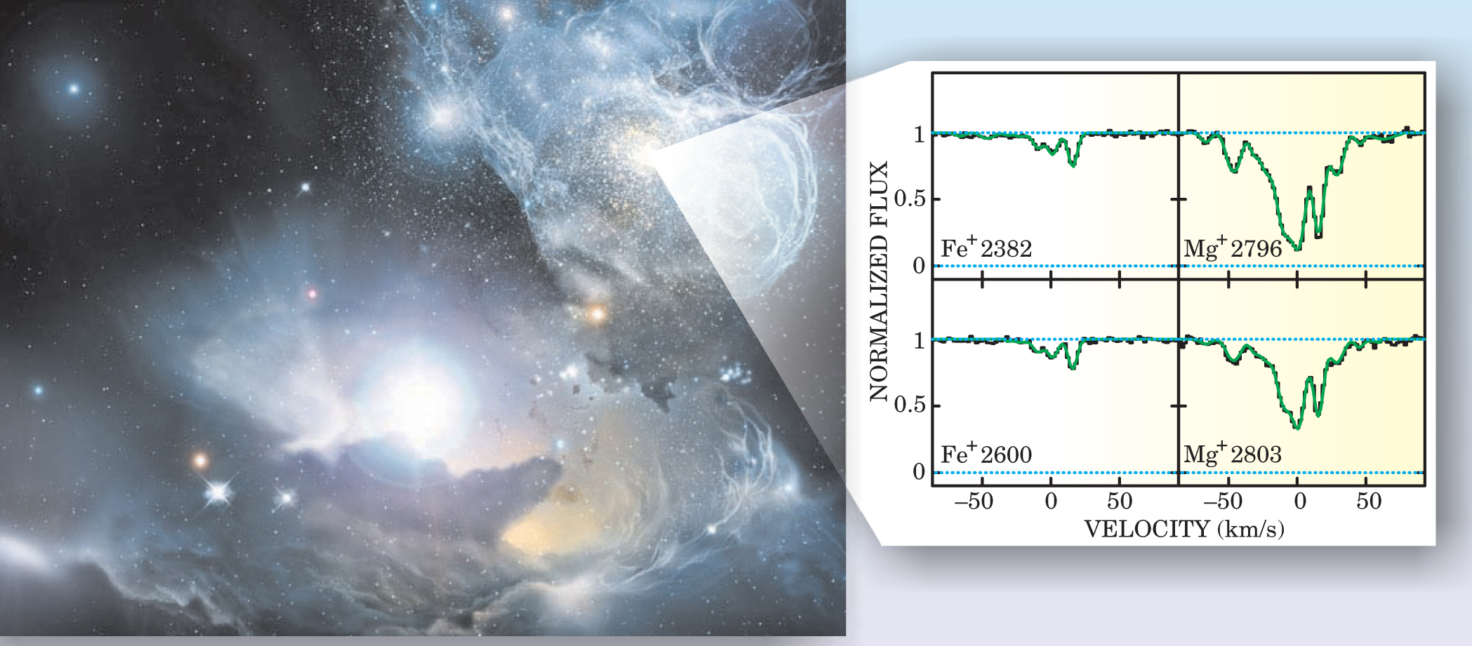
Observations 4,5 of quasar absorption systems (see figure 1) at cosmological redshifts z = 0.5–3.0 have piqued interest in the idea that the fundamental constants of nature vary in time. After comparing several transition lines from several elemental species (we offer technical details and further discussion below) James Webb, Michael Murphy, Victor Flambaum, and colleagues reported the statistically significant result Δα/α = (−5.4 ± 1.2) × 10−6. The negative sign means that the past value of α is smaller than the present value. Inspired by that provocative result, we concentrate in this article mainly on possible variations of the fine-structure constant.

A gaseous cloud lies along the line of sight to a distant quasar in this artist’s rendition. The iron and magnesium spectra (green; the cosmological redshift is 1.3) on the right both show subtle variations when different lines are compared. By studying such variations for a variety of elements, scientists can probe for changes in the fine-structure constant over cosmological timescales. Velocities in the spectra are given relative to an arbitrary standard.
(Drawing courtesy of Wolfram Freudling et al., Space Telescope–European Coordinating Facility, ESO, ESA, and NASA; spectra adapted from M. T. Murphy et al., http://arXiv.org/abs/astro-ph/0310318.)
Various sensitive experimental checks constrain the variation of coupling constants. 6 Limits can be derived from cosmology (from both Big Bang nucleosynthesis 7 and the microwave background 8 ), the Oklo natural reactor in Gabon, 9 long-lived isotopes found in meteoritic samples, 10,11 and atomic clock measurements. 12–14
Cosmological bounds
The theory of Big Bang nucleosynthesis describes the production, in the early universe, of the light isotopes deuterium, helium-3, helium-4, and lithium-7. Its success relies on, among other things, a fine balance between the overall expansion rate of the universe, proportional to (G N N)1/2 where N is the number of relativistic particles, and the weak interaction rates that control the relative number of neutrons to protons at the onset of nucleosynthesis. Changes in the weak rates—which may result from changes in fundamental parameters—or a change in the expansion rate affects the neutron to proton ratio and ultimately the 4 He abundance. Thus, one can use the concordance between theory and the observed light-element abundances to constrain the physics of models that go beyond the standard model.
As described in
The theoretical prediction for Y agrees with observation to within a few percent, which allows one to deduce that the relative change in a over the 13-billion-year history of the universe has been no more than about 5%. Assuming a constant rate of change over that time, that result is equivalent to 1/α | dα/dt | ≲ 4 × 10⁻¹²/yr over the past 13 × 109 years.
In the context of unified or string-inspired theories, in which the strong, weak, and electromagnetic gauge couplings come together at a so-called unification scale, one can derive significantly stronger limits on the variation of α. At energies above the unification scale, those theories are characterized by a single gauge constant. At energies below the unification scale, each of the three gauge constants has its own energy dependence, and so the three are distinguishable. Thus, in unified theories, a change in the fine-structure constant implies a change in other couplings. The dominant effects are found in induced variations of Λ QCD and ν. Because those quantities have dimensions, we are implicitly referring to variations with respect to some fixed mass scale such as the Planck mass, M P = (ℏc/G N)1/2.
Exactly how changes in the fine-structure constant are related to changes in the QCD and weak-interaction scales depends on theoretical details, but typically one finds ΔΛ QCD /Λ QCD ≈ 30Δα/α and Δν/ν ≈ 100Δα/α. The Higgs mechanism generates masses that are proportional to ν for all quarks and leptons and also for the weak gauge bosons W and Z. Variations in Λ QCD and ν translate to variations in all low-energy particle masses. In short, if α varies in unified or string-inspired theories, virtually all masses and couplings likely vary as well, typically much more strongly than the variation induced by changes in the Coulomb interaction alone. As a consequence, the nucleosynthesis bound on α, for example, improves by about two orders of magnitude in unified scenarios.
One can also derive cosmological bounds based on measurements of the microwave background. As the universe expands, its radiation cools to the “decoupling” temperature T dec, at which protons and electrons can combine to form neutral hydrogen atoms. Once those neutral atoms are in place, photons are decoupled from the protons and electrons. At decoupling, when the universe was some 400 000 years old, exp(–E b/T dec) was roughly equal to the number ratio of baryons (that is, protons and neutrons) to photons, about 6 × 10⁻¹⁰. Measurements of the microwave background can determine the decoupling temperature to within a few percent, which in turn determines E b at decoupling. Because changes in α lead to changes in E b, the fine-structure constant can have changed by at most a few percent since decoupling.
A simple extended gravity theory
The construction of theories with variable “constants” is straightforward. Consider a gravitational Lagrangian that includes ΦR as one of its terms, where Φ is a scalar field and R is the Einstein curvature scalar. The gravitational constant is determined if the dynamics of the theory fix the expectation value of the scalar field 〈Φ〉. That is, in units for which ℏ = c = 1,
So-called Jordan-Brans-Dicke theories are specific realizations in which scalar fields allow for the possibility of a time-varying gravitational constant. Such theories, however, can always be reexpressed in a way that keeps G N fixed and shunts the time dependence to other mass scales through their dependence on the scalar field. For example, a simple JBD action can be written as
When the action is expressed as above, an evolving scalar field Φ leads to a varying G N. However, the JBD action can be expressed in terms of the conformally related metric
In this representation, Newton’s constant is constant, but the fermion mass varies as 〈Φ〉−1/2 (one needs to rescale ψ) and the cosmological constant varies as 1/〈Φ〉2. The physics does not depend on how the action is represented, and, in particular, the measurable dimensionless quantity Gm 2 ∝ 1/〈Φ〉 is independent of representation.
In the theory described here, the fine-structure constant remains constant. But it is easy enough to construct theories in which it, too, varies. For example, a Lagrangian term ΦF 2 that couples a scalar field to the electromagnetic field tensor fixes the fine-structure constant to be
Big Bang nucleosynthesis of 4He
The helium-4 abundance can be estimated simply from the ratio of the neutron to proton number densities, n/p, by assuming that essentially all free neutrons are incorporated into 4He. Thus the mass fraction Y of 4He is
When neutrons and protons are in chemical equilibrium, their relative abundance is determined by the usual Boltzmann exponential. Neutrons and protons cease to be in chemical equilibrium after the temperature falls to the so-called freeze-out temperature, T f ≈ 0.8 MeV, at which the weak interaction rate for interconverting neutrons and protons falls below the expansion rate of the universe. At that time, the neutron to proton ratio is given by
Reactors and meteorites
Two billion years ago, in the southeast of Gabon, a natural fission reactor operated at what is now the Oklo uranium mine. By studying the observed isotopic abundance distribution at Oklo—for example, the ratio of samarium-149 to samarium-147—one can derive constraints on the variation of α.9
The Sm isotopic ratio is of special interest because it can be related to the cross section for the radiative neutron capture of 149Sm to yield an excited state of 150Sm. That cross section, in turn, depends sensitively on the resonance energy E r for the capture. The observed isotopic ratios at Oklo determine the value E r had 2 billion years ago, which can be compared to the current value of 0.0973 eV. The change in the resonance energy | ΔE r/E r | ≲1 can then be related to a change in α.
One contribution to the resonance energy comes from the Coulomb energy E C = (3/5)(e 2/r 0)Z 2/A 1/3, where Z is the number of protons in the nucleus, A – Z the number of neutrons, and r 0 = 1.2 femtometers. The Coulomb contribution clearly scales with α. If all the change in the resonance energy can be attributed to a change in the Coulomb term, then |ΔE r| = 1.16|Δα/α| MeV, from which one can obtain the limit |Δα/α| ≲ 10−7. Allowing all fundamental couplings to vary interdependently yields the more stringent limit |Δα/α| < 5 × 10⁻¹⁰.
Precise meteoritic data coupled with present laboratory measurements of the decay rates for the long-lived isotopes rhenium-187, uranium-235, and uranium-238 constrain the beta-decay rate of 187Re back to the time of solar system formation—about 4.6 billion years ago. 11 Armed with those constraints, one can derive limits on possible variations of the fine-structure constant at a redshift of 0.45 or so. That redshift value borders the range of redshifts over which observations of quasar absorption systems suggest variations in α. The pioneering studies on the effect of variations of fundamental constants on radioactive decay rates were performed by James Peebles and Robert Dicke and by Freeman Dyson. 10
The β-decay rate λ is proportional to some power n of the energy Q released during the decay. As with the resonant energy for neutron capture, the Coulomb energy E C contributes to Q. As a consequence, changes in α are related to changes in decay rates.
Isotopes with the lowest Q are typically most sensitive to changes in α because Δλ/λ = n(ΔQ/Q) is large for small Q. The isotope with the smallest Q (2.66 ± 0.02 keV) is 187Re, which decays into osmium-187. If some radioactive 187Re were incorporated into a meteorite formed in the early solar system, the present abundance of 187Os in the meteorite would be (187Os)0 = (187Os)i + (187Re)0[exp (λ 187 t) –1], where the subscripts i and 0 denote the initial and present abundances respectively; λ 187 is the decay rate for 187Re; and t is the meteorite’s age.
A plot of the present abundance of 187Os (divided by the present abundance of 188Os, which does not receive any decay contributions) versus the present abundance of 187Re (likewise normalized to 188Os) for samples gathered from iron meteorites gives a straight line. From the slope of that line, one can precisely determine the product λ 187 t.
The technique of correlating 187Re with 187Os can be applied to other parent–daughter pairs to derive the product of the relevant decay rate and meteoric age. Because the alpha-decay rates of 238U and 235U are rather insensitive to variations in fundamental couplings, the decay rates of those isotopes, as determined from laboratory measurements, along with correlations of uranium-isotope abundances to the amount of lead-206 and lead-207 precisely determine the age of angrite meteorites to be 4.558 billion years.
The iron meteorites containing 187Re were formed within 5 million years of the angrite meteorites. From the U–Pb age of those meteorites and the slope of the Re–Os line, one can precisely determine λ 187.
The derived value of λ 187 covers decay over the past 4.6 billion years. By comparing it with the present value of the decay rate, as measured in the laboratory, one can limit the variation of α to Δα/α = (8 ± 8) × 10−7. Again, if one allows all fundamental couplings to vary interdependently, a more stringent limit, Δα/α = (2.7 ± 2.7) × 10−8, may be obtained.
Atomic clocks
Measurements of transition frequencies in atomic clocks have set impressive bounds on the variation of a over the past several years. Those experiments consider two kinds of transition: electronic transitions, in which the spatial wavefunctions of electrons change, and hyperfine transitions during which only the total spin of the electron and nucleus changes.
The electronic transition frequency ν el depends on a relativistic correction F, which is a function of α and the atom undergoing the transition. The hyperfine transition frequency ν hf depends on (µ/µ B)α 2 F, where µ is the nuclear magnetic moment of the relevant atom and µ B is the Bohr magneton. For atoms X and Y,
If one supposes that the Bohr magneton and all magnetic moments are fixed so that only α can vary, then either of the frequency ratios given above can be used to probe for changes in α.
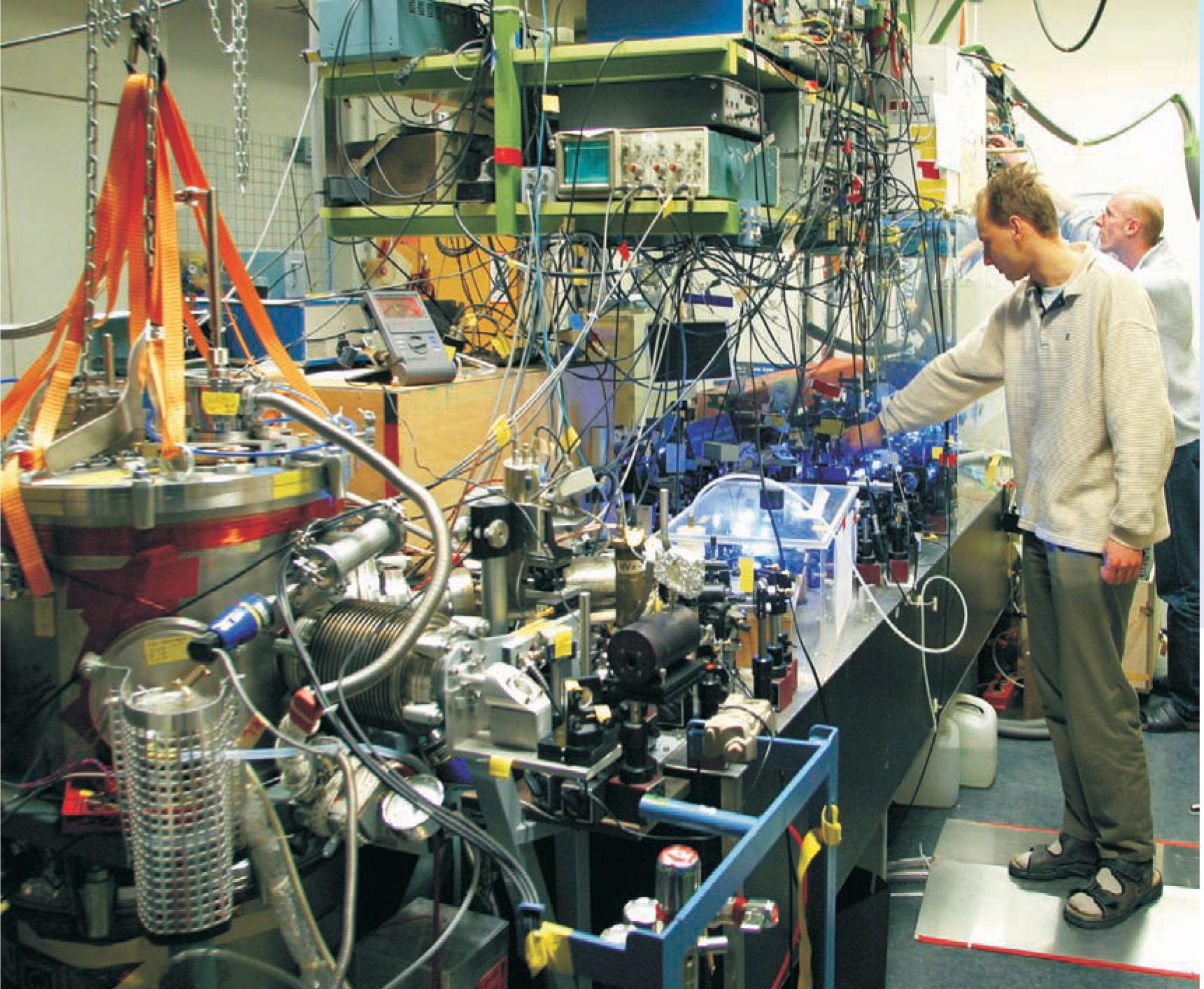
Three experiments conducted over the past several years have led to markedly improved constraints on the recent variation of α. Measurements comparing hyperfine transitions in rubidium-87 and cesium-133 over a four-year period 12 have established the limit | Δα/α | < 5 × 10⁻¹⁵. A three-year observation 13 of the electric quadrupole transition in singly charged mercury-199 and of the ground-state hyperfine transition of 133Cs determined that | Δα/α | < 4 × 10⁻¹⁵. A third experiment (see figure 2) compared the hyperfine transition in 133Cs to 1S–2S electronic transitions in atomic hydrogen. Independent electronic-transition measurements taken 3.6 years apart determined that Δα/α = (−4.1 ± 8.2) × 10−15 over that period. 14

Electronic transitions in hydrogen, when compared with hyperfine transitions in cesium-133, constrain variations in the fine-structure constant. The hydrogen beam apparatus is visible in the front of this experiment, which was conducted at the Max Planck Institute for Quantum Optics in Garching, Germany. Behind the apparatus, Nicolai Kolachevsky (forefront) and Marc Fischer adjust the laser system.
(Courtesy of Theodor Hänsch.)
The data from the two experiments that compared hyperfine and electronic transitions can be combined, which allows one to consider generalized scenarios in which µ/µB , in addition to α, may vary. The combined data constrain the recent variations in the fine-structure constant to (1/α)dα/dt = (0.9 ± 2.9) × 10−15/yr.
Alkali doublets and many multiplets
The line of sight to a distant, high-redshift quasar is often blocked by absorption clouds. The quasar acts as a bright source, and the absorption features seen in its spectra reflect the clouds’ chemical abundances.
Consider a doublet absorption feature involving, for example, S 1/2 → P 3/2 and S 1/2 → P 1/2 transitions. The overall wavelength position of the doublet is a measure of the red-shift of the absorption cloud, but the relative line splitting δλ/λ (with λ the line’s wavelength) is a measure of the fine-structure constant. To relate the line splitting to α, recall that the energy splitting due to the spin–orbit coupling is
The relative energy splitting δE/E ∝ δλ/λ ∝ α 2. Thus, any change in the relative line spacing between quasar and terrestrial spectra is proportional to Δα/α.
The more complicated many-multiplet method compares transitions from different multiplets and different atoms and utilizes the effects of relativistic corrections to the spectra.
Quasars
Much of the excitement over the possibility of a time-varying fine-structure constant stems from a series of recent observations of quasar absorption systems. In those observations, the so-called many-multiplet method was applied to several transition lines from several elemental species. A key part of the technique, which uses relativistic corrections to the atomic transition spectra frequencies, is to compare spectra whose line shifts are particularly sensitive to changes in α with spectra that don’t display such behavior. The comparison allows one to determine Δα/α with a sensitivity of order 10−6.
At relatively low redshift (z < 1.8), the crucial comparison is between iron and magnesium (representative line spectra for those elements are shown in figure 1). At higher redshifts, an iron–silicon comparison is most important, although in all cases the analysis includes other elemental transitions. Webb and coworkers 5 applied the many-multiplet method to data, taken by the high-resolution echelle spectrometer (HIRES) on Mauna Kea’s Keck I telescope, with redshifts that ranged from about 0.5 to about 3.0. They reported a statistically significant variation in the fine-structure constant Δα/α = (–5.4 ± 1.2) × 10−6.
More recent observations taken with the ultraviolet and visual echelle spectrograph (UVES) at the European Southern Observatory’s Very Large Telescope have not duplicated the Webb result. A many-multiplet analysis 15 of several Fe lines from a single source found Δα/α = (0.1 ± 1.7) × 10−6. It is not clear, however, that the single-source Fe result contradicts the Webb result, which relied on a statistical average of more than 100 absorbers and whose data had significant scatter. A more significant disagreement arose from a study 16 that compared Mg and Fe lines in a set of 23 systems. That experiment set a limit on the possible variation of the fine-structure constant Δα/α = (–0.6 ± 0.6) × 10−6.
Although less sensitive than the many-multiplet method, the related alkali-doublet method may also be used to test for variability in α. The relatively simple physics behind the approach is described in
The results reported in reference and those based on the statistically dominant subsample of low redshift absorbers described in reference are sensitive to the assumed isotopic abundance ratio of Mg. Both research groups took the Mg abundances to have the same ratios as found in the Sun. That is, they took 24 Mg: 25 Mg: 26 Mg = 79:10:11. They further argued, based on then current studies of galactic evolution, that their estimates of the heavy-isotope abundances were, if anything, high: Had they assumed that only 24 Mg was present in the quasar absorbers, they noted, they would have obtained significantly different results. The UVES data would have yielded Δα/α = (–3.6 ± 0.6) × 10−6 and the low-redshift subsample of the HIRES data would have given Δα/α = (–9.8 ± 1.3) × 10−6.
The sensitivity to Mg isotopic ratios of results derived from Fe–Mg systems has led one of us (Olive), Grant Matthews, and Timothy Ashenfelter to offer a new interpretation of the many-multiplet analyses. 18 Rather than indicating a variation of α, they may be explained in terms of the early nucleosynthesis of 25 Mg and 26 Mg. Those heavy isotopes are efficiently produced in intermediate mass stars, particularly those with masses 4–6 times the mass of the Sun, when helium and hydrogen are burning in shells outside the carbon and oxygen core. According to this new interpretation, the many-multiplet method traces the chemical history of primitive absorption clouds. The hypothesis will be tested by future observations and examinations of correlations among other heavy elements produced in intermediate-mass stars.
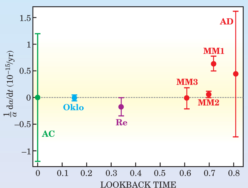
Most physicists take for granted the constancy of fundamental physical constants. However, whether those constants change with time is not just a philosophical question—it can be discussed in plausible theoretical frameworks. Even more important, it has been addressed by a number of observations and experiments. Figure 3 summarizes some of the results discussed in this article. Although most observations and experiments provide constraints on the variation of the fine-structure constant, recent observations of quasar absorption systems have indicated a statistically significant variation. That’s an exciting and important result. Does it truly represent a variation of the fine-structure constant or does it have an alternative interpretation in the intricate chemical evolution of the universe? Time will tell.

A variety of experiments look for possible changes in the fine-structure constant α over times spanning much of the age of the universe. In this plot, normalized time derivatives, assumed to be constant, are graphed against the lookback time, the fraction of the universe’s age that has elapsed between the time of the plotted point and the present. The results summarized come from a representative atomic clock (AC) measurement (from reference
References
1. M. J. Duff, L. B. Okun, G. Veneziano, J. High Energy Phys. 2002(03), 023 (2002).https://doi.org/10.1088/1126-6708/2002/03/023
See also M. J. Duff, http://arXiv.org/abs/hep-th/0208093 ;
G. F. R. Ellis, J.-P. Uzan, http://arXiv.org/abs/gr-qc/0305099 .2. L. B. Okun, Sov. Phys. Usp. 34, 818 (1991).https://doi.org/10.1070/PU1991v034n09ABEH002475
3. B. Bertoti, L. Iess, P. Tortora, Nature 425, 374 (2003).https://doi.org/10.1038/nature01997
4. J. K. Webb et al., Phys. Rev. Lett. 82, 884 (1999);https://doi.org/10.1103/PhysRevLett.82.884
M. T. Murphy et al., Mon. Not. R. Astron. Soc. 327, 1208 (2001);https://doi.org/10.1046/j.1365-8711.2001.04840.x
J. K. Webb et al., Phys. Rev. Lett. 87, 091301 (2001);https://doi.org/10.1103/PhysRevLett.87.091301
M. T. Murphy et al., Mon. Not. R. Astron. Soc. 327, 1223 (2001).https://doi.org/10.1046/j.1365-8711.2001.04841.x5. M. T. Murphy, J. K. Webb, V. V. Flambaum, Mon. Not. R. Astron. Soc. 345, 609 (2003).https://doi.org/10.1046/j.1365-8711.2003.06970.x
6. Two good reviews are P. Sisterna, H. Vucetich, Phys. Rev. D 41, 1034 (1990), andhttps://doi.org/10.1103/PhysRevD.41.1034
J.-P. Uzan, Rev. Mod. Phys. 75, 403 (2003).https://doi.org/10.1103/RevModPhys.75.4037. E. W. Kolb, M. J. Perry, T. P. Walker, Phys. Rev. D 33, 869 (1986);https://doi.org/10.1103/PhysRevD.33.869
B. A. Campbell, K. A. Olive, Phys. Lett. B 345, 429 (1995);https://doi.org/10.1016/0370-2693(94)01652-S
S. Sarkar, Rep. Prog. Phys. 59, 1493 (1996);https://doi.org/10.1088/0034-4885/59/12/001
L. Bergstrom, S. Iguri, H. Rubinstein, Phys. Rev. D 60, 045005 (1999);https://doi.org/10.1103/PhysRevD.60.045005
K. A. Olive, G. Steigman, T. P. Walker, Phys. Rep. 333, 389 (2000);https://doi.org/10.1016/S0370-1573(00)00031-4
K. Ichikawa, M. Kawasaki, Phys. Rev. D 65, 123511 (2002);https://doi.org/10.1103/PhysRevD.65.123511
K. M. Nollett, R. E. Lopez, Phys Rev. D 66, 063507 (2002).https://doi.org/10.1103/PhysRevD.66.0635078. G. Rocha et al., New Astron. Rev. 47, 863 (2003).https://doi.org/10.1016/j.newar.2003.07.018
9. A. I. Shlyakhter, Nature 264, 340 (1976);https://doi.org/10.1038/264340a0
T. Damour, F. Dyson, Nucl. Phys. B 480, 37 (1996);https://doi.org/10.1016/S0550-3213(96)00467-1
Y. Fujii et al., Nucl. Phys. B 573, 377 (2000);https://doi.org/10.1016/S0550-3213(00)00038-9
K. A. Olive et al., Phys. Rev. D 66, 045022 (2002).https://doi.org/10.1103/PhysRevD.66.04502210. P. J. Peebles, R. H. Dicke, Phys. Rev. 128, 2006 (1962);https://doi.org/10.1103/PhysRev.128.2006
F. J. Dyson, in Aspects of Quantum Theory, A. Salam, E. P. Wigner, eds., Cambridge U. Press, New York (1972), p. 213.11. M. Linder et al., Geochim. Cosmochim. Acta 53, 1597 (1989);https://doi.org/10.1016/0016-7037(89)90241-X
G. W. Lugmair, S. J. G. Galer, Geochim. Cosmochim. Acta 56, 1673 (1992);https://doi.org/10.1016/0016-7037(92)90234-A
M. I. Smoliar et al., Science 271, 1099 (1996);https://doi.org/10.1126/science.271.5252.1099
K. A. Olive et al., Phys. Rev. D 69, 027701 (2004).https://doi.org/10.1103/PhysRevD.69.02770112. H. Marion et al., Phys. Rev. Lett. 90, 150801 (2003).https://doi.org/10.1103/PhysRevLett.90.150801
13. S. Bize et al., Phys. Rev. Lett. 90, 150802 (2003).https://doi.org/10.1103/PhysRevLett.90.150802
14. M. Fischer et al., http://arXiv.org/abs/physics/0311128 ;
M. Fischer et al., http://arXiv.org/abs/physics/0312086 .15. R. Quast, D. Reimers, S. A. Levshakov, http://arXiv.org/abs/astro-ph/0311280 .
16. H. Chand et al., Astron. Astrophys. 417, 853 (2004); R. Srianand et al., Phys. Rev. Lett. 92, 121302 (2004).
17. M. T. Murphy et al., Mon. Not. R. Astron. Soc. 327, 1237 (2001);https://doi.org/10.1046/j.1365-8711.2001.04842.x
A. F. Martinez Fiorenzano, G. Vladilo, P. Bonifacio, Mem. Soc. Astron. Ital. 3 (Supp.), 252 (2003);
J. N. Bahcall, C. L. Steinhardt, D. Schlegel, Astrophys. J. 600, 520 (2004).https://doi.org/10.1086/37997118. T. P. Ashenfelter, G. J. Mathews, K. A. Olive, Phys. Rev. Lett. 92, 041102 (2004); see also http://arXiv.org/abs/astro-ph/0404257 .https://doi.org/10.1103/PhysRevLett.92.041102
More about the authors
Keith Olive is the director of the William I. Fine Theoretical Physics Institute and a Distinguished McKnight University Professor and Yong-Zhong Qian is an associate professor and a McKnight Presidential Fellow; both are in the school of physics and astronomy at the University of Minnesota, Minneapolis.
Keith A. Olive, University of Minnesota, Minneapolis, US .
Yong-Zhong Qian, University of Minnesota, Minneapolis, US .


