Wall-bounded turbulence

In his classic 1971 text, Peter Bradshaw refers to turbulence as “the most common, the most important and the most complicated kind of fluid motion.” ¹ Now, more than 40 years later, the claim remains easily justifiable. Turbulence is likely familiar to anyone who has flown on an airplane or watched water rush past a rock in a stream. It emerges in any number of natural and manmade settings, from atmospheric and oceanic currents to flows in pipelines and heat exchangers. It influences weather, pollution levels, and climate change and figures into the design of propulsion devices, wind turbines, clean rooms, artificial hearts, and irrigation systems.

The complexity of turbulence is evidenced by the fact that after more than a century of concerted research effort, many of its seemingly simple questions remain unanswered. It has been said, in fact—in a quote variously ascribed to Arnold Sommerfeld, Albert Einstein, and Richard Feynman—that “turbulence is the last great unsolved problem of classical physics.” Part of the complexity stems from the fact that turbulent flows are composed of recurrent, sometimes coherent flow structures, or eddying motions, that exhibit a range of length scales spanning several orders of magnitude, all interacting with one another.

The problem becomes still more complex when the flow is confined by one or more solid surfaces. The presence of a wall introduces new length scales and fundamentally changes the nature of turbulence. Although the biggest changes are limited to the thin layer near the surface, that layer is of outsized practical importance. For example, the behavior of that near-wall region largely determines the drag force on a plane or ship, the distribution of heat in the atmosphere, and the energy required to deliver oil and other goods through pipelines. Consider that according to the US Department of Transportation, in 2009 the 409 000 miles of pipelines in the US carried 21% of all ton-miles of freight. For perspective, the US Energy Information Administration estimates that the environmental impact of reducing transportation energy by 5% would be equivalent to that of doubling the US wind energy production.

Our understanding of wall-bounded turbulent flows has developed rather slowly. But recent advances in computational and experimental capabilities have delivered new insights that may finally break the logjam. Experiments at a handful of new facilities across the globe have revealed new scaling and universalities in wall-bounded flows, which in turn hold promise to vastly increase the kinds of problems we can solve computationally—and the efficiency with which we can solve them.

Viscosity and inertia

In the simplest case, a turbulent flow is characterized by a competition between viscous forces, which damp out velocity fluctuations by dissipating kinetic energy into heat, and inertia forces, which tend to generate and preserve velocity fluctuations. The ratio of inertia to viscous forces is known as the Reynolds number, Re = UL/ν, where U and L are characteristic velocity and length scales and ν is the kinematic viscosity of the fluid.

If Re is less than 10 or so, inertia forces are negligible and the flow is laminar and more or less perfectly damped. The velocity field adjusts almost instantly to any changes in the pressure gradients that drive the flow. Such is the flow regime experienced by swimming bacteria and dust particles in air.

In the intermediate range 10 < Re < 10³, inertia forces become increasingly important, though not strong enough to give rise to persistent velocity fluctuations. Included in that category of laminar flow are capillary and pulmonary flows in the human body and gliders in air or in water.

At Re > 10³, however, viscous effects may not be strong enough to damp out velocity disturbances introduced into the flow field. As a result, a tiny fluctuation—due to, say, a small roughness element or surface vibration—may grow to the point that it causes the entire flow to destabilize.

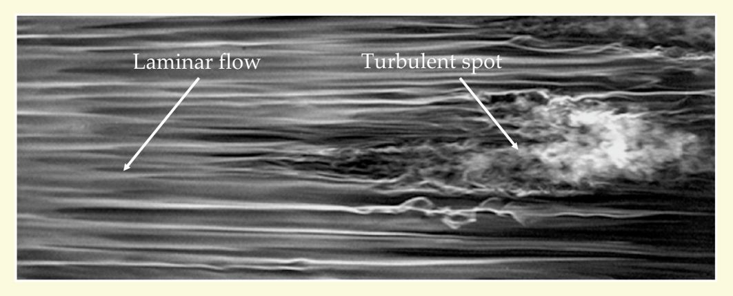
Figure 1 shows one common form of disturbance growth, a spreading patch of turbulence called a turbulent spot, in air flowing over a flat plate. Small velocity fluctuations in the flow far from the plate generate a turbulent spot near the plate’s surface. The spot grows with downstream distance until it encompasses the entire flow domain. In such a flow, bound on one side by a surface, turbulence is confined to a finitely thick region above the surface known as a boundary layer.

The turbulent flow field is marked throughout by irregular velocity and pressure fluctuations. The magnitude of the velocity fluctuations may be as large as 10–50% of the time-averaged velocity. The fluctuating velocity field can be viewed as a collection of eddies of varying length scales. ² As we’ll see, the nature of the eddies is important in determining the statistical properties of the flow.

Eddies, great and small

Consider the canonical example of a flow through a pipe. If we are far downstream from the entrance to the pipe, and if the inlet conditions are steady, then the flow statistics become independent of downstream distance, and the flow is said to be fully developed. Molecular-scale forces at the fluid–wall interface ensure that the velocity of the fluid at the wall is equal to the velocity of the wall itself; the wall is said to impose a no-slip boundary condition. If y is the distance from the wall and the pipe is our reference frame, then both u, the instantaneous streamwise velocity, and ū, the time average of that velocity, are zero when y = 0.

What does the velocity profile look like away from the wall? If the flow is laminar, ū varies smoothly, as a parabola, with y. As shown in figure 2a, ū is greatest at the pipe’s centerline. In a turbulent flow, however, eddies very effectively mix momentum—as well as heat and mass—and significantly increase energy dissipation. That tends to reduce the velocity gradients in the bulk and, because the no-slip boundary condition must still be obeyed, increase the gradients near the wall.

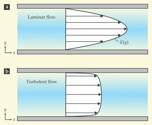
The result is a profile like the one shown in figure 2b, in which the velocity gradients near the wall are much larger than they would be in a laminar flow. Viscous forces, which are proportional to velocity gradients, are also especially large in the near-wall region of a turbulent flow. They exert upon the wall what’s known as skin-friction drag, a key component of the resistance felt by an object—be it a ship, fish, or plane—as it moves through a fluid. Skin-friction drag also influences the energy required to pump fluid through a pipe. In general, the more turbulent a flow is, the more energy will be lost due to the effects of the skin-friction drag.

The wall also affects the distribution of a turbulent flow’s energy. In the classical picture of turbulent flow, kinetic energy is introduced into the system in the form of large eddies. For pipe flows, the largest eddies scale with pipe radius R and can extend to lengths in excess of 10R. In a channel, the largest eddies scale with the channel width; in a boundary-layer flow, they scale as the thickness of the turbulent layer.

In what’s known as an energy cascade, energy is transferred from large eddies to progressively smaller ones—usually by a mechanism called vortex stretching. Such cascades are thought to occur without significant energy loss—dissipative viscous forces are negligible at large scales—and the process is sometimes referred to as inertial transfer.

Eventually, the eddies become small enough to be destroyed by viscous dissipation. That length scale sets the minimum eddy size and is known as the Kolmogorov length scale η. Interestingly, the length scales associated with the largest and smallest eddies give rise to an alternative definition of the Reynolds number, Re_η = (R/η)^4/3.

For wall-bounded flows, we prefer to define the Reynolds number in terms of τ_w, the frictional shear stress the fluid exerts on the wall, both because τ_w is experimentally measurable and because it is an important parameter for many applications. At the centerline of a pipe flow, the Kolmogorov length scale η can be estimated as (Rν³/u_τ³)^1/4, where u_τ = (τ_w/ρ)^1/2 is the so-called friction velocity and ρ is the density of the fluid. Hence the Reynolds number becomes Re_τ = u_τR/ν.

The energy-cascade description assumes that the most energetic eddies are much larger than the least energetic ones—that is, that Re_η and Re_τ are large. Although that assumption fairly describes the bulk portion of most wall-bounded flows, it breaks down in the near-wall region. There, even the most energetic eddies are relatively small, on the order of η. In fact, because the turbulent energy in a wall-bounded flow is typically supplied by the wall, there can exist a reverse energy cascade, from small to large scales.

The laws of the wall

Directly solving or computing the flow field of turbulent flows is a difficult endeavor. However, scaling arguments can yield valuable insights into the behavior of canonical flows—or at least certain regions of those flows—and allow one to identify important flow characteristics using a relatively small number of nondimensional parameters. Throughout much of the 20th century, the focus of scaling arguments was on understanding the behavior of velocity and turbulent momentum transport in the near-wall region.

Turbulent momentum transport can be expressed in terms of Reynolds stresses, mathematical products of velocity fluctuations. In the pipe flow, for example, the quantity ρu′u′, where u′ = u − ū, corresponds to a streamwise Reynolds stress. (Other important Reynolds stresses in a pipe flow are ρv′v′ ρw′w′, and ρu′v′, where v′ and w′ are velocity fluctuations in the wall-normal and cross-stream directions.)

Near the wall, Reynolds stresses must go to zero and thus momentum transport is dominated by viscous forces. In that so-called inner region, the relevant velocity and length scales are u_τ and ν/u_τ; the nondimensional wall distance is y⁺ = yu_τ/ν; and the nondimensional streamwise velocity is u⁺ = ū/u_τ. In the outer region of the flow, we expect momentum transport to be dominated by Reynolds stresses (although viscous forces do remain important for energy dissipation at very small scales). The relevant length scale becomes that of the largest eddies, R. Velocity, meanwhile, can still be scaled by u_τ, which is related to the wall stress and therefore affects the entire profile.

In the 1930s Clark Millikan proposed that if the inner region is much thinner than the outer one, there may exist an overlap region—a “(possibly) small but finite region near the wall” ³ where both the inner and outer scalings apply. Using dimensional and overlap arguments, he showed that the mean velocity profile in the overlap region should follow a logarithmic law: u⁺ = κ⁻¹ ln y⁺ + C, where the constant C depends on details of the flow, but κ, known as von Kármán’s constant, is thought to be universal. The result is the same one that was deduced by Ludwig Prandtl in 1925. (Here, we’ve nondimensionalized according to the inner-region length scale; an expression nondimensionalized according to the outer-region length scale takes a similar form.) Millikan’s result has received widespread experimental support. ⁴

In the 1970s, Alan Townsend recognized that in the overlap region the Reynolds stress ρu′u′ behaves in a similar way, in the sense that both the inner and outer scalings apply. Townsend argued that the eddies in the overlap region are essentially attached to the wall—their size scales accordingly with their distance y. ⁵ Summing over the contributions from those attached eddies, Townsend predicted that the Reynolds stress should follow its own logarithmic law: u′u′⁺ = u′u′/u_τ² = B − A ln(y/R), where the constant B depends on the details of the flow, but A is expected to be universal. (Again, although we’ve nondimensionalized according to the outer-region length scale, an expression nondimensionalized according to the inner-region length scale takes a similar form.)

Unlike the log law of velocity, the early evidence in support of Townsend’s law of Reynolds stresses was rather circumstantial. Both derivations rest on the assumption of a large separation of length scales—that is, large Re_τ. Indeed, for many real flows—including flows past ships and planes and atmospheric flows across the Earth’s surface—Re_τ is on the order of 10⁴–10⁶ (see figure 3). Until recently, however, even state-of-the-art experimental facilities could achieve at most Re_τ ~ 5 × 10³—sufficient to see hints of Townsend’s log law but not to definitively confirm it. (Some atmospheric boundary-layer experiments can achieve Re_τ of order 10⁶, but the experimental challenges are numerous and the data tend to be of poorer quality.) In the 1990s there was a major push to establish facilities capable of achieving higher Re flows. And that is where the story of wall-bounded turbulence takes a new and exciting turn.

At the frontiers of turbulence

In the march toward higher Reynolds numbers, three experimental facilities were especially noteworthy: the Princeton University Superpipe, which uses compressed air as the working fluid; the large boundary-layer wind tunnel at the University of Melbourne in Australia; and the Large Cavitation Channel, an immense water tunnel established by the US Navy in Memphis, Tennessee. Around the turn of the century, those facilities began yielding high-precision measurements of near-wall velocity and stress profiles at Re_τ of order 10⁵.

Results from a Princeton experiment are shown in figure 4 and clearly exhibit the logarithmic profile of streamwise Reynolds stresses predicted by Townsend. Moreover, the logarithmic portions of the velocity and turbulent-stress profiles coincide in space. That universality was previously suspected, but has only now been confirmed.

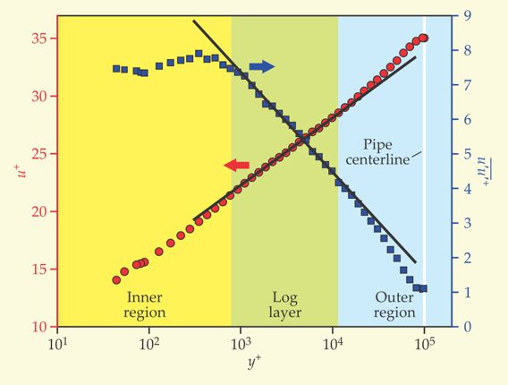
A few features of the plot deserve a closer look. First, the inner region is remarkably thin, less than 1% of the pipe radius. Second, Reynolds stresses are larger in the inner region than in the outer one—an indication that turbulent momentum transport is strongest near the wall. Because those stresses must equal zero at the wall, the data suggest that a peak in turbulent momentum transport lies in the inner region. Other experiments, ⁴ not shown, indicate that the peak remains fixed at y⁺ ≈ 12 as Re_τ increases. At the same time, the scaling of the Reynolds stress indicates that the logarithmic region makes an increasingly important (and eventually dominant) contribution to the overall energy balance.

Viscous forces, on the other hand, are always strongest near the wall, but they decay quickly with increasing distance from it. As Re_τ grows, the viscosity-dominated region becomes increasingly thin and increasingly difficult to resolve in experiments and computations.

New physics, new computations

Ultimately, scaling laws like those derived by Millikan and Townsend tell only part of the story of turbulent wall-bounded flow. To obtain a more detailed picture and to describe flows with more complicated geometries, one typically must turn to computation.

The ideal approach is to numerically solve the system’s momentum and mass balances, the Navier–Stokes and continuity equations, respectively. In direct numerical simulation (DNS), one solves those equations at grid points on a mesh; reliable results require a mesh size comparable to the smallest length scale of motion in the system. Thus, capturing the spatial fluctuations of a three-dimensional turbulent flow requires on the order of Re_τ^9/4 grid points. Capturing the fluctuating field in time and accounting for additional computing overhead ⁶ requires computer resources that scale nominally as Re_τ⁴. Considering many real-world flows have Re_τ > 10⁶, the computing costs associated with DNS can quickly become prohibitive.

At the other end of the computing spectrum are what’s known as Reynolds-averaged Navier–Stokes (RANS) methods, which solve time-averaged versions of the Navier–Stokes and continuity equations. The Reynolds stresses due to velocity fluctuations are then calculated based on empirical models. Fast and cheap, RANS methods are the workhorse of industry. But they can be unreliable when applied to flows for which the Reynolds-stress models haven’t been calibrated.

Large eddy simulation (LES) is a middle way: It solves the complete Navier–Stokes and continuity equations for large-scale motions and then invokes an empirically determined effective viscosity to describe forces at the smallest scales. Because LES captures much of the unsteady and 3D nature of turbulence, it can describe many practical flows with a greater fidelity than RANS.

However, when a wall is present the LES grid is typically constrained by the near-wall region, where turbulent and viscous momentum transport occur on small scales (see figure 5a). As a result, for wall-bounded flows the computational costs of LES are estimated to scale as Re_τ^1.8, only a modest savings over DNS. ⁷ If, instead, one could empirically model the flow in the near-wall layer (see figure 5b), the grid requirements could be greatly relaxed, which would lead to a significant payoff; it’s estimated that the computational costs would scale as Re_τ^0.2.

In the 1970s James Deardorff ⁸ and Ulrich Schumann ⁹ independently attempted to develop such wall-layer models. They approximated the boundary conditions based on time-averaged properties of the logarithmic region. That general approach is still in use today in various forms, but because it doesn’t account for the time-dependent nature of turbulent interactions, it has achieved limited success in describing high-Re flows (Re_τ > 10⁴).

Here insights from high-Re experiments—in Princeton and Melbourne and at the University of Illinois at Urbana-Champaign—should be helpful. Those studies all revealed unexpected flow structures known as very large scale motions ² or superstructures, ¹⁰ which extend as far as 10–30 R in the streamwise direction in pipe flow. At high Re, those superstructures can contribute up to 20% of the turbulent kinetic energy of a pipe flow.

What can those motions tell us about the much smaller eddies near the wall? We have postulated that the near-wall motions follow a universal behavior, independent of the flow geometry, and that those motions are modulated by the superstructures, such that the actual velocity field at the wall is a superposition of the near-wall-eddy and superstructure velocity fields. ¹¹ Indeed, measurements suggest that the superstructures so impose a very low frequency modulation on the near-wall velocity fluctuations. Crucially, the parameters of the superposition and modulation can likely be derived from the velocity signature in the logarithmic layer.

Efforts toward implementing the wall-layer model into LES are ongoing, but preliminary results are encouraging and have shown trends that are in line with experimental evidence. ¹² The approach holds promise for extending the computationally accessible Re range up to that of atmospheric boundary-layer experiments.

Another valuable aspect of such wall-layer models is that they elucidate the connection between superstructures and the intensity of the local wall stress. Such information could plausibly reveal new strategies to reduce drag by manipulating the superstructures, which are more accessible inputs for control schemes than the near-wall motions that have been targeted in the past.

Zettaflops and yottabytes

Advances in camera, laser, and computing technologies have vastly improved our ability to obtain time-resolved velocity fields and other information about the dynamics of high-Re flows. However, DNS remains an important tool for generating high-fidelity, fully 3D data that are difficult to obtain experimentally. Moreover, DNS will continue to serve as a benchmark for new measurement techniques and new LES models.

To date, DNS of wall-bounded turbulence has been limited to relatively low Re_τ, at most around 4 × 10³. (A simulation at Re_τ = 5 × 10³ by Robert Moser and colleagues, currently ongoing, promises to set a new record.) A tentative consensus is that simulations at Re_τ = 10⁴ would probably be sufficient to answer many of the field’s open questions—and that threshold could conceivably be reached before the end of this decade. Still, it is interesting to consider the computing resources required to carry out DNS at the high values of Re_τ currently achievable in experiments.

According to calculations by Javier Jiménez ¹³ that were adjusted to reflect the decreasing memory-to-computing speed ratio in high-performance computers, one would need more than 10 zettaflops (10 × 10²¹ floating-point operations per second) of computing power to complete a DNS at Re_τ = 10⁵ in a typical time. According to the TOP500 project, ¹⁴ the world’s fastest computer can perform at just onemillionth that speed, at about 33 petaflops. Assuming computing speed continues to grow at its current exponential rate, DNS at Re_τ = 10⁵ won’t become feasible until roughly 2035.

Even if high-Re simulations do become realizable in the coming decades, tools for processing and handling large data sets will need to keep up. DNS simulations at Re_τ = 10⁴ and Re_τ = 10⁵ would generate 23 terabytes and 23 petabytes of data per time step, respectively. Simulating the required 10⁷ time steps at Re_τ = 10⁵ would produce around 0.2 yottabytes—more digital content than currently exists in the entire world.

Clearly, storing all of that information would be neither feasible nor desirable. Simulating high-Re flows will require selective storage of data as they are being generated, which in turn will require a high-level appreciation of the physics. The same applies to laboratory and field studies, where the rapidly increasing size of data sets generated in 3D, time-resolved experiments is becoming a major issue. The process will likely be an iterative and evolving one, with the ultimate goal being to formulate high-fidelity empirical models.

Gathering momentum

In this article we have focused on relatively simple, canonical wall-bounded turbulent flows. Other challenges emerge if one wants to model turbulent flows having additional parameters or complications such as compressibility, shock waves, multiple phases, combustion, density jumps, body forces due to pressure gradients, and magnetic fields. Each problem presents specific challenges, but a common thread remains: the need to understand how various-sized eddies emerge, evolve, and interact in the flow.

In the coming years, computational, experimental, and modeling efforts should continue to produce new advances. Computing resources will undoubtedly continue to improve, although those changes will also require new approaches and technologies for handling vast data sets. New experimental facilities will also be important, and at present several such facilities are either under construction or under development, including sulfur fluoride tunnels in Göttingen, Germany; the CICLoPE pipe facility in Predappio, Italy; and a turbulent convection facility in Ilmenau, Germany.

Turbulence has been the focus of concerted research efforts since the work of Osborne Reynolds more than a century ago, and the general study of the topic dates back even further. The field’s recent advances bode well for the foreseeable future, and we anticipate—and certainly hope—that the mysteries of turbulence will not have to wait yet another century to be solved.

References

1. P. Bradshaw, An Introduction to Turbulence and Its Measurement, Pergamon Press, New York (1971), p. xi.
2. R. J. Adrian, Phys. Fluids 19, 041301 (2007). https://doi.org/10.1063/1.2717527
3. C. B. Millikan, in Proceedings of the Fifth International Congress for Applied Mechanics, J. P. D. Hartog, H. Peters, eds.,Wiley, New York (1939), p. 386.
4. A. J. Smits, B. J. McKeon, I. Marusic, Annu. Rev. Fluid Mech. 43, 353 (2011). https://doi.org/10.1146/annurev-fluid-122109-160753
5. A. A. Townsend, The Structure of Turbulent Shear Flow, 2nd ed., Cambridge U. Press, New York (1976).
6. V. Yakhot, K. R. Sreenivasan, J. Stat. Phys. 121, 823 (2005). https://doi.org/10.1007/s10955-005-8666-6
7. U. Piomelli, E. Balaras, Annu. Rev. Fluid Mech. 34, 349 (2002). https://doi.org/10.1146/annurev.fluid.34.082901.144919
8. J. W. Deardorff, J. Fluid Mech. 41, 453 (1970). https://doi.org/10.1017/S0022112070000691
9. U. Schumann, J. Comp. Phys. 18, 376 (1975). https://doi.org/10.1016/0021-9991(75)90093-5
10. N. Hutchins, I. Marusic, J. Fluid Mech. 579, 1 (2007). https://doi.org/10.1017/S0022112006003946
11. I. Marusic, R. Mathis, N. Hutchins, Science 329, 193 (2010). https://doi.org/10.1126/science.1188765
12. M. Inoue, R. Mathis, I. Marusic, D. I. Pullin, Phys. Fluids 24, 075102 (2012). https://doi.org/10.1063/1.4731299
13. J. Jiménez, J. Turbulence 4, N22 (2003).
14. TOP500 List–June 2013, http://www.top500.org/list/2013/06 .
15. M. Matsubara, P. H. Alfredsson, J. Fluid Mech. 430, 149 (2001). https://doi.org/10.1017/S0022112000002810
16. M. Hultmark, M. Vallikivi, S. C. C. Bailey, A. J. Smits, Phys. Rev. Lett. 108, 094501 (2012). https://doi.org/10.1103/PhysRevLett.108.094501
More about the authors
Alexander Smits is the Eugene Higgins Professor of Mechanical and Aerospace Engineering at Princeton University in Princeton, New Jersey, and a professorial fellow at Monash University in Victoria, Australia. Ivan Marusic is an Australian Research Council Laureate Fellow and a professor of mechanical engineering at the University of Melbourne in Melbourne, Australia.