Time-reversal methods in geophysics
DOI: 10.1063/1.3480073
Before the 20th century there were few seismometers. So Earth’s dynamic geophysical processes were poorly understood. Today the potential for understanding those processes is enormous: The number of seismic instruments is continually increasing, their data are easily stored and shared, and computing power grows exponentially. As a result, seismologists are rapidly discovering new kinds of seismic signals in the frequency range 0.001-100 Hz, as well as relatively large nonseismic displacements, monitored by the global positioning system, occurring over days or weeks.
Such new signals manifest geophysical events very different from classical earthquakes. A classical earthquake occurs when one crustal block slips past another at a fault surface (see the

Figure 1. Seismic signals. Seismometers detect dynamic displacements by monitoring the three components of acceleration or velocity over a wide frequency range. (a) A classical earthquake. During the first 3000 seconds after a 7.0-magnitude earthquake struck Haiti in 2010, the record of north-south acceleration at a seismometer 3800 km away is dominated by the surface waves arriving at around 1300 s. But the blowup shows the earlier arrival of the much weaker bulk waves: the P wave at 400 s and the S wave at 730 s. (b) A glacial earthquake. In this broadband record (0.1 to 20 Hz) of the vertical velocity component at a seismic station about 150 km from the quake, a slowly varying substructure is almost obscured by high-frequency noise. (c) Tremor. Shown here is the vertical component of acceleration recorded at a seismic station in California following the magnitude-7.9 Alaska earthquake of 2002. The blowup, from which all frequencies below 3 Hz are filtered out, reveals a noiselike, very-low amplitude-signal with a 22-s period that corresponds to the Love-wave period. This “driven tremor” is broadcast from an unknown source driven by passage of the Love wave. Glacial quakes and tremor signals have, in general, no identifiable P- or S-wave arrivals.
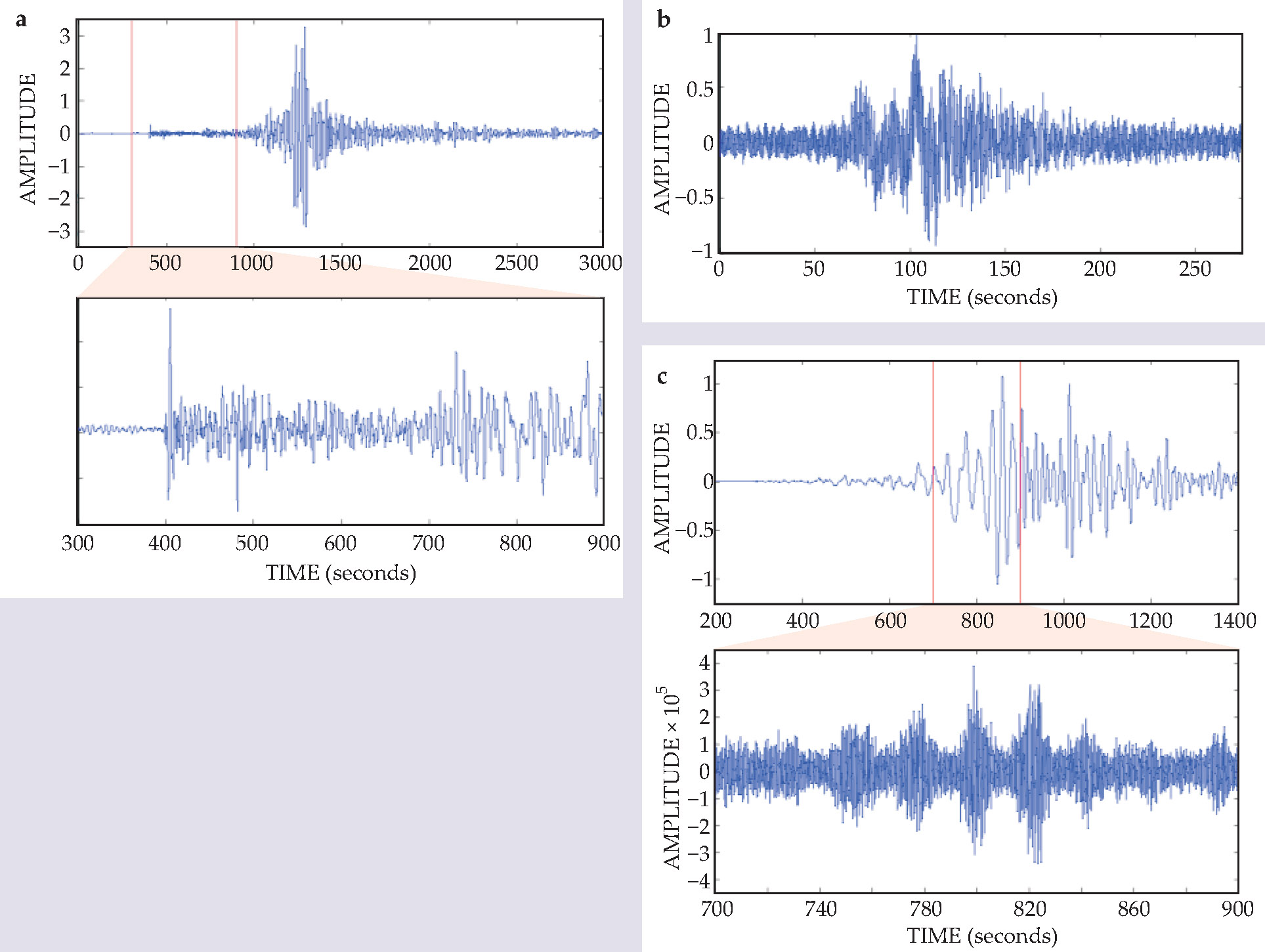
A principal goal of geophysics is to translate signal features such as spatial and temporal structure and amplitude into Earth motions. Location, as determined by comparing signals arriving at dispersed detectors, is a primary issue. For instance, pinpointing a classical earthquake places it in a specific plate-tectonic setting. Its radiation pattern indicates how the fault blocks moved—for example, subduction or strike-slip. Spatial and temporal signal structure let seismologists estimate the stress released by the earthquake and assess the prospects for subsequent seismic activity—in particular, strong ground shaking, the most dangerous consequence of earthquakes and an essential input for civil engineering and architecture.
The new kinds of events, subjects of intense investigation, offer the promise of additional insight into Earth processes. The observation of episodic tremor and slip in the Cascadia subduction zone of the US and Canadian Pacific Northwest constrains estimates of the extent of the locked segment of the zone’s fault system. That segment, which last ruptured in 1700 at magnitude 9, threatens Seattle and Vancouver.
Glacial earthquakes and Earth hum are coupled to atmospheric conditions and thus serve as proxies for monitoring climate. The locations, signal structures, and depths of seismic sources are relevant to monitoring for violations of the nuclear nonproliferation treaty. For example, a shallow event with a spherically symmetric radiation pattern is almost certainly an explosion, whereas a deep event with a strike-slip radiation pattern is presumably an earthquake.
Classical earthquakes are relatively easy to locate by triangulation, which relies on the ability to identify the arrivals of P and S waves (see the
Location by time reversal
For the new event types, source location is more challenging.
4
In general, they exhibit no identifiable P- and S-wave arrivals. The tremor signal in figure
Beyond seismology, time-reversal methods, described early in their development by Mathias Fink in Physics Today (March 1997, page 34 ), have emerged as powerful tools for employing acoustic and elastic waves in signal processing, imaging, and the inspection of materials. 5–7 Imagine a movie of a pebble dropped into a pond, ripples moving outward. Stop the movie and run it backward to the moment of the pebble drop. That thought experiment contains the essential recipe for TR. The movie run forward, from pebble drop to ripple arrival at some location on the pond, is the recipe’s forward part. The second step, the movie run backward to the pebble drop, is the time-reversed part.
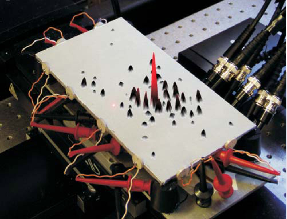
Translated into an experimental protocol, the recipe is illustrated in figure 2. In the experiment shown, eight transducers spaced around the periphery of an aluminum plate record the arrivals of signals propagated from a vertical blow delivered near the center of the plate’s underside. The transducers then rebroadcast time reversals of the received signals back into the plate. The result, monitored on the plate by a laser vibrometer, exhibits local peaks. The largest peak correctly reveals the location of the instigating blow. Smaller peaks are due to reflections and the incomplete coverage of the periphery by the transducers.

Figure 2. Time reversal in the lab. A source on the underside of a thin aluminum plate, near its center, emits a 20-µs strain pulse. The resulting displacements arriving at the plate’s edges are recorded by eight detectors arrayed along the perimeter. The recorded signals are time-reversed and rebroadcast from the detectors. A laser vibrometer scans the plate’s surface and maps the vertical component of its velocity due to vibrations created by the rebroadcast. The superposed peaks display the velocity map at the moment when the rebroadcast signals focus to reveal the original source (red peak). The lesser peaks are due to reflections and other secondary sources.
(Adapted from
Of course, when playing the pond-ripple movie backward, you rebroadcast much more information than can this experiment, with its discrete transducer network. In the movie, a point on the pond’s surface is first passed by the concentric ripples from the pebble drop, then by ripples scattered from a protruding rock, later by ripples that encountered bulrushes, and later still by ripples that scattered off obstacles farther out. Over time, multiple propagation paths provide more and more information about the source.
A sparse set of detectors is a make-do surrogate for the reversed-movie ideal. When the signals impinging on a detector site are time-reversed, they unfold in reversed sequence as they return to the source. When time-reversed, any arbitrary time segment will return to the source. Therefore TR methods don’t need identifiable timing features.
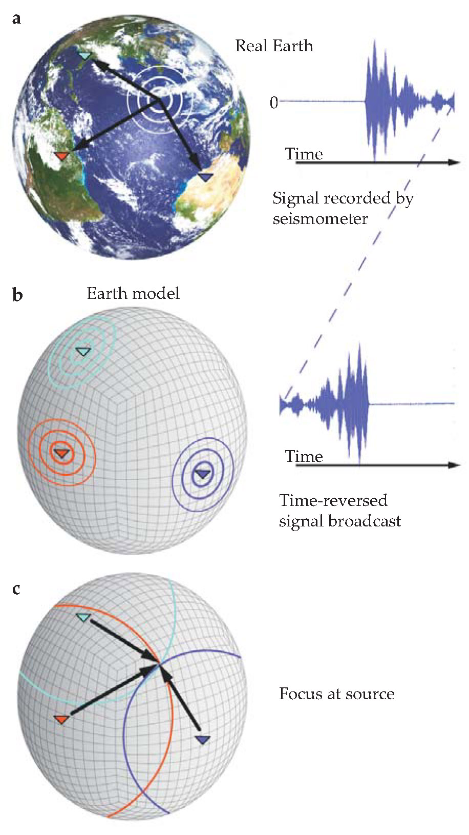
How is the TR recipe implemented in geophysics? An unknown source broadcasts a signal that is then received at a set of seismic stations. In the illustration in figure 3, seismic signals arriving at different times at three stations are recorded. In a computer simulation, the signals are time-reversed and rebroadcast from their respective stations into a model of the elastic structure of Earth. Such Earth models specify propagation velocity as a function of position. The TR wakefield in the Earth model is then examined for focusing, which should reveal the location and nature of the source.

Figure 3. Time-reversal seismology. (a) A seismic signal radiating from its source is recorded by three distant stations. (b) The signals are time-reversed and, in a computer simulation, rebroadcast from their respective stations into a model Earth. (c) The time-reversed signals propagating through the model Earth converge at a focus, revealing the location and structure of the real source.
There are three important ingredients in numerical implementation of the TR recipe: the set of seismic stations, the velocity model, and the choice of “imaging fields” chosen for inspecting the results. The velocity model probably introduces the greatest uncertainty. Velocity models are created by aggregating any information that will help — for example, local borehole data and, on larger scales, propagation-time data from seismic events. A promising recent development in the honing of velocity models is the so-called adjoint model, which involves differences between real seismic signals and models for those signals. 8 The development of increasingly reliable velocity models is an ongoing quest.
Geophysical applications
Let us describe several examples of TR methods in geophysics. The first use of TR for source location was made in the early 1980s. Using ideas that grew out of seismic signal—processing schemes for hydrocarbon exploration, George McMechan and colleagues at the University of Texas at Dallas assembled the essential ingredients of the TR method. 9 They successfully imaged the source of a small 1983 aftershock earthquake in California. Their purely acoustical rebroadcast was into a two-dimensional model of a 15-by-12-km vertical slice of the formation that contained the seismic stations and the suspected source. That first application revealed the limitations imposed by the seismic-station set, the velocity model, and computing power.
Geophysical lexicon
Fault motions. (a) A strike-slip fault like the San Andreas fault in California involves two blocks sliding past each other at an approximately vertical interface. (b) At a subduction zone, blocks slide past each other at a roughly horizontal interface. In the Pacific Northwest, for example, the Juan de Fuca tectonic plate slides eastward under the North American plate.
Radiation patterns. (c) A lurch at a point on a strike-slip fault launches elastic waves with displacement polarity varying around the source. Regions that gain or lose material in the process are marked, respectively, by + or −. The elastic-wave radiation pattern elucidates the nature of the lurch. (d) By contrast, an explosive source, such as an underground nuclear weapons test, launches a symmetrical radiation pattern with the same displacement phase in all directions. (e) A lurch at a subduction zone is intrinsically much like a strike-slip lurch. But its elastic-wave broadcast pattern looks very different on the surface.
Waves. (f) Earth’s elastic bulk transmits compressional waves (P waves) and shear waves (S waves). (g) Surface waves, strongly excited by near-surface sources, also come in two varieties: Rayleigh waves are largely compressional, and Love waves are pure shear waves. The surface waves generally dominate seismic signals. They decay exponentially with increasing depth. (Adapted from ref. .)

More recent applications of TR exhibit the fruits of great advances in all three limiting factors. 10 Figure 4 shows a result from a TR study of the 2004 magnitude-9 Sumatra earthquake. 11 That cataclysmic event was caused by a rupture of about 1200 km that moved from south to north along the Indonesian subduction zone over about seven minutes. It was recorded by seismic stations around the world.

Figure 4. The great Sumatra earthquake of 2004. The quake, lasting about 400 s, resulted from a 1200-km-long rupture between tectonic plates. Seismic records from 165 stations worldwide were time-reversed and rebroadcast into a model Earth. The three maps, each extending from Siberia to Australia, show the propagation of the vertical displacement field thus deduced in reverse time order, labeled by time t since the quake’s onset. Blue and red indicate, respectively, upward and downward displacements. The contracting time-reversed wave field begins collapsing onto the extended fault at about 400 s.
(Adapted from
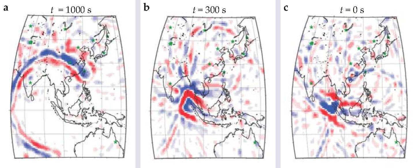
The signals recorded at 165 stations over a time interval of 8000 s (long enough to record surface waves circling the planet in opposite directions) were time-reversed and rebroadcast into a whole-Earth velocity model. Figure 4 shows the resulting last 1000 s of the time-reversed return of the displacement field to its extended source. As the wavefront returns to the source region beginning at about 400 s, the focus moves from north to south, showing the history of the rupture in reverse order. From figure
Figure 5 shows a TR result from a 2001 magnitude-5 glacial earthquake in Greenland. 12 The seismic signals, recorded at 146 stations over 4000 s, were filtered to include only frequency components from 0.01 to 0.02 Hz (periods of one or two minutes), which carry most of the information from glacial earthquakes. The filtered time trains were time-reversed and rebroadcast into an Earth velocity model. The figure shows the surface velocity field thus deduced for southern Greenland at t = 0, the instant of the quake’s onset.

Figure 5. For a glacial earthquake in Greenland, vertical-displacement signals recorded at 146 seismic stations worldwide were frequency-filtered, time-reversed, and rebroadcast into a model Earth to produce these surface-velocity fields for southern Greenland at the moment of focus, which in the time-inverted record corresponds to the instant of the quake’s onset. (a) The absolute-velocity field |v| indicates two sources near opposite ends of a glacier on Greenland’s east coast. (b) The vz field, which maps the vertical component of surface velocity at the quake’s onset, reveals that the eastern source, near the glacier’s front, was thrusting down while the western source, near its upstream end, was thrusting upward.
(Adapted from
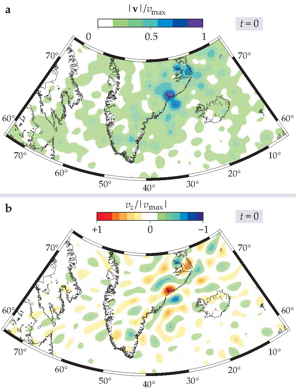
The velocity-magnitude field (figure
A TR wave-propagation scheme typically yields the vector displacement field u. That field can be used in various ways, as the Greenland glacial-quake analysis shows. Additional useful information can often be gleaned by examining derivative imaging fields such as
The new event types
Glacial earthquakes, Earth hum, and meteorological events such as hurricanes belong to the event set that defines “environmental seismology,” a term coined by French geophysicist Jean-Paul Montagner. With seismic signatures that don’t have the timing signature of classical earthquakes, they are all candidates for TR methods.
Among the new event types, tremor is the most enigmatic. In 2002, geophysicist Kazushige Obara observed tremor along the subducting Philippine Sea plate near Japan. 3 That initial observation of tremor has been followed by many more. Roughly speaking, tremor is a low-amplitude, noiselike signal in the frequency range 1-10 Hz. At a single station, tremor appears amidst the noise and looks unremarkable. It becomes evident as a seismic event when the noise signals recorded at several stations far apart are found to be correlated in time.
In the example of figure
Locating and characterizing the source of tremor broadcasts by TR methods is not easy. The frequencies that carry the interesting information, around 5 Hz, are high by seismological standards. Therefore, the typical wavelengths that must be reliably rebroadcast into a model Earth are small—on the order of a kilometer. So the simulation codes must grid relevant segments of the model Earth on length scales as small as 0.1 km. Such calculations make heavy demands on computational resources. Furthermore, tremor sources are weak, and they are often seen at only a few stations. The considerable effort that has been invested in TR methods for tremor source location has thus far met with only limited success.
Virtual sources
Beyond locating and characterizing seismic sources, TR methods have other uses in geophysics. A notable example is the possibility of exploiting broadcasts from so-called virtual sources. In the laboratory experiment illustrated in figure 2, a source driven vertically sends to transducers on the perimeter signals of displacements in the plane of the plate—that is, orthogonal to the source displacement. The reciprocity of the Green’s function for elastodynamics implies that the in-plane response on the perimeter to a vertical drive at the center must be the same as the vertical response at the center to in-plane drives on the perimeter. Thus one could broadcast from each perimeter transducer, record the signal received at the center, time-reverse it, and broadcast it from the original source transducer. That would result in signals that converge on the center and then diverge from it as if a true source were located there. The center has become a virtual source.
That scenario can be used to explore geological formations when, for instance, the perimeter detectors are a set of surface transducers surrounding a down-hole receiver. A virtual source is created at the down-hole receiver when broadcasts from the surface are detected and time-reversed at the down-hole receiver, and then rebroadcast from the surface transducers. Recently Andrey Bakulin and coworkers have used that scheme for imaging beneath a seismically opaque geologic stratum. 17
A powerful tool
We have described how TR methods applied to the 2004 Sumatra earthquake showed the devastating event unfold backward in time, revealing its extended source and the direction of its rupture. Application of TR to a glacial earthquake revealed its source and evidence of the forces to which it subjected the surface.
In cases such as glacial earthquakes and tremors, obscure timing signatures can sometimes be extracted from complex seismic signals. Those signatures yield useful limits on duration and frequency content. In principle, TR methods can use any portion of the tremor wavefront for a rebroadcast that reveals the locations and characteristics of sources.
The successful application of TR methods depends on adequate coverage by seismic stations, reliable velocity models, and sufficient computational resources. As those crucial resources continue to improve, TR will find growing application as a powerful tool in the suite of methods for elucidating seismic processes.
This work was supported by the Laboratory Directed Research and Development program at Los Alamos National Laboratory.
References
1. G. Ekström, M. Nettles, G. Abers, Science 302, 622 (2003). https://doi.org/10.1126/science.1088057
2. N. Suda, K. Nawa, Y. Fukao, Science 279, 2089 (1998) https://doi.org/10.1126/science.279.5359.2089
T. Tanimoto et al., Geophys. Res. Lett. 25, 1553 (1998), https://doi.org/10.1029/98GL01223.3. K. Obara, Science 296, 1679 (2002). https://doi.org/10.1126/science.1070378
4. D. Shelly et al., Nature 442, 188 (2006); https://doi.org/10.1038/nature04931
H. Kao et al., Nature 436, 841 (2005). https://doi.org/10.1038/nature039035. M. Fink et al., Proc. IEEE Ultrasonics Symp. (Montreal) 1, 681 (1989);
M. Fink, Contemp. Phys. 37, 95 (1996); https://doi.org/10.1080/00107519608230338
C. Draeger, M. Fink, Phys. Rev. Lett. 79, 407 (1997). https://doi.org/10.1103/PhysRevLett.79.4076. B. E. Anderson et al., Acoust. Today 4(1), 5 (2008). https://doi.org/10.1121/1.2961165
7. M. Fink, G. Montaldo, M. Tanter, Annu. Rev. Biomed. Eng. 5, 465 (2003). https://doi.org/10.1146/annurev.bioeng.5.040202.121630
8. J. Tromp, C. Tape, Q. Liu, Geophys. J. Int. 160, 195 (2005). https://doi.org/10.1111/j.1365-246X.2004.02453.x
9. G. A. McMechan, Geophys. J. R. Astron. Soc. 71, 613 (1982); https://doi.org/10.1111/j.1365-246X.1982.tb02788.x
G. A. McMechan, J. Luetgert, W. Mooney, Bull. Seismol. Soc. Am. 75, 1005 (1985).10. D. Gajewski, E. Tessmer, Geophys. J. Int. 163, 276 (2005); https://doi.org/10.1111/j.1365-246X.2005.02732.x
A. Rietbrock, F. Scherbaum, Geophys. J. Int. 119, 260 (1994). https://doi.org/10.1111/j.1365-246X.1994.tb00926.x11. C. Larmat, et al., Geophys. Res. Lett. 33, L19312 (2006), https://doi.org/10.1029/2006GL02336.
12. C. Larmat, J. Tromp, Q. Liu, J. -P. Montagner, J. Geophys. Res. 113, B09314 (2008), https://doi.org/10.1029/2008JB005607 .
13. J. Gomberg, et al., Science 319, 173 (2008). https://doi.org/10.1126/science.1149164
14. G. Rogers, H. Dragert, Science 300, 1942 (2003). https://doi.org/10.1126/science.1084783
15. F. Bregnuier, et al., Science 321, 1478 (2008). https://doi.org/10.1126/science.1160943
16. L. Me´tivier, et al., Earth Planet. Sci. Lett. 278, 370 (2008).
17. A. Bakulin, R. Calvert, Geophysics 71(4), SI139 (2006); https://doi.org/10.1190/1.2216190
V. Korneev, A. Bakulin, Geophysics 71(3), A13 (2006). https://doi.org/10.1190/1.219686818. For more detail, see http://web.ics.purdue.edu/~braile/edumod/waves/WaveDemo.htm .
More about the authors
Carène Larmat is a postdoctoral geophysicist at Los Alamos National Laboratory in New Mexico. Robert Guyer, emeritus professor of physics at the University of Massachusetts Amherst, is affiliated with Los Alamos and the University of Nevada, Reno. Paul Johnson is a geophysicist at Los Alamos.
Carène S. Larmat, 1 Los Alamos National Laboratory, New Mexico, US .
Robert A. Guyer,, 2 University of Massachusetts Amherst, US .
Paul A. Johnson, 3Los Alamos, US .


