The physics of river prediction
DOI: 10.1063/PT.3.4523


Rivers support life and fuel civilization. 1 , 2 They provide water for drinking, irrigate food crops, and help build everything from cars to computers. Their waters drive hydroelectric turbines that generate clean energy. Rivers have even supported nuclear physics developments that changed the course of a war: The hydroelectric complexes of the Columbia Basin Project and the Tennessee Valley Authority enabled energy-intensive uranium and plutonium refinement for the Manhattan Project.
Rivers have always been crucial transportation pathways. The exploration, settlement, and economic development of the Americas depended acutely on river navigation. The Danube serves as a trade route in Europe, much as it did for the Romans 2000 years ago, and today it carries commercial freight across the continent.
Rivers also provide homes for precious ecosystems. They house fisheries, facilitate recreation, and bring in tourism dollars. That’s not to mention their tremendous cultural value: American literature wouldn’t be the same without Mark Twain’s recollections of his experiences as a Mississippi riverboat pilot.
Rivers can also kill. Floods are the most devastating natural force in the US, and at times they have been architects of history. In 1948, the Columbia River flooded and wiped out the progressive Portland suburb of Vanport, Oregon. Fifteen people died, and the destruction permanently changed the area’s racial dynamics. The flood also motivated the US and Canada to negotiate the Columbia River Treaty, intended in part to support flood control efforts. Droughts are subtler than floods but are considered more damaging globally.
Although the water wars predicted in 1995 by then World Bank vice president Ismail Serageldin are unlikely to materialize, 3 competition over scarce water resources has occasionally led to violence. For example, Israeli and Syrian forces skirmished in the mid 1960s over water resources in the Jordan River basin.
Predicting variability and long-term changes in river flows, like those shown in figure
Figure 1.

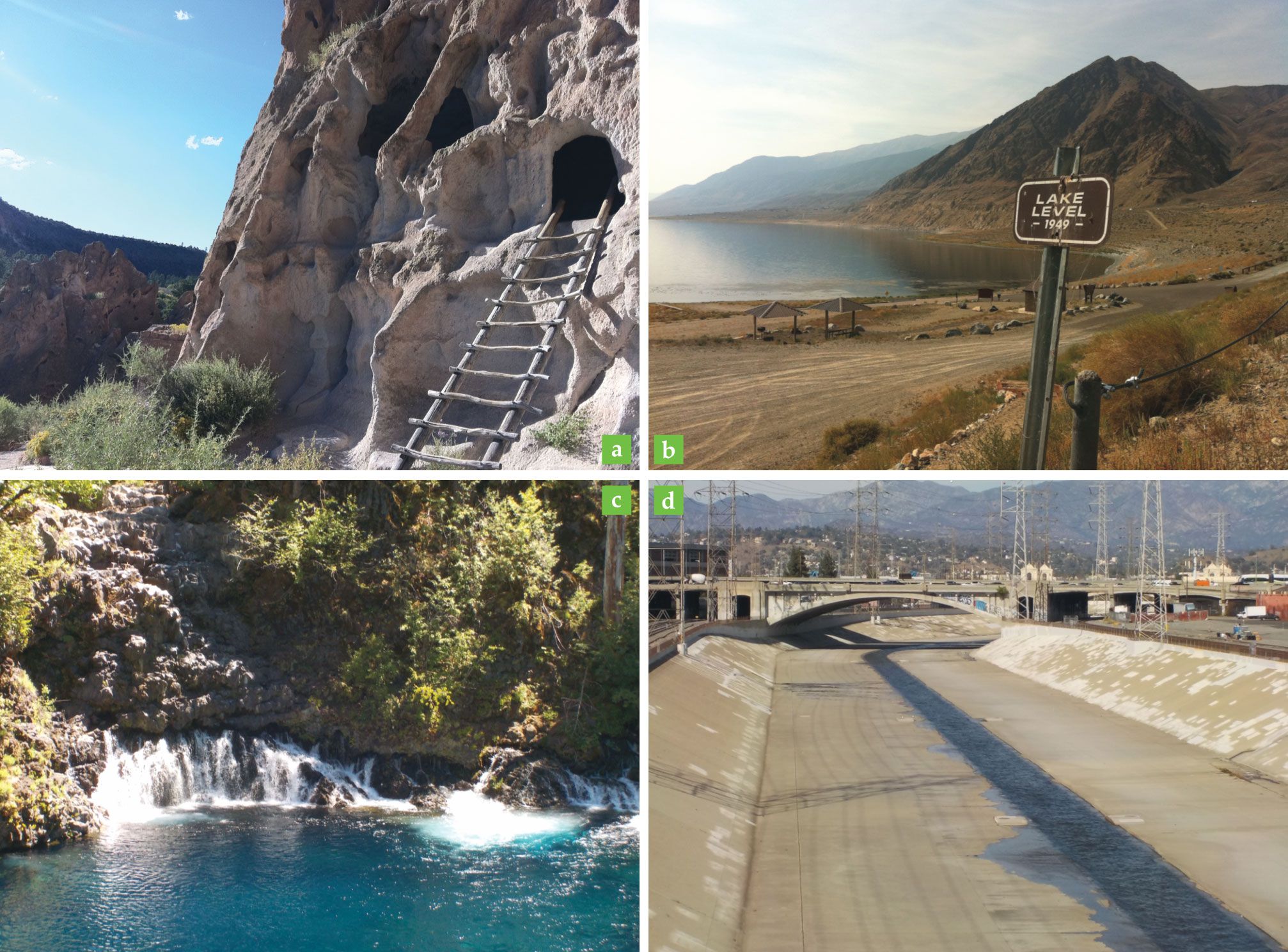
Rivers and other water resources evolve in response to natural and anthropogenic factors. (a) The advanced society that lived in Ancestral Puebloan (formerly known as Anasazi) ruins near Los Alamos, New Mexico, moved on around 1200 AD, in part because of the drying climate. (b) Nevada’s Walker Lake is a remnant of ice-age Lake Lahontan; its water level has dropped 55 m since the 19th century, mainly from diversions for agriculture. (c) The McKenzie River springs from a volcanic aquifer at Tamolitch Falls in the Oregon Cascades in a dramatic demonstration of river–aquifer interactions. Accurately capturing the water-storage effects can be crucial for river-flow forecasting. (d) The Los Angeles River is a favorite filming location for car chases in Hollywood movies. Such highly urbanized rivers no longer have the natural water storage and release mechanisms seen in the McKenzie River. They are therefore more variable and flood-prone, which makes accurate forecasting even more crucial—and more challenging. (Photos by Sean Fleming.)
How do watershed hydrology models work, and what physical principles do they embody? Each model can include contributions from numerous disciplines: civil engineering, geophysics, agricultural engineering, meteorology, climate science, glaciology, and others. Given that complexity, how do hydrologists pick which systems and processes to include in their models? How do they choose appropriate representations and implement them effectively? What, in short, is the physics behind river-prediction models?
What’s under the hood?
River prediction models are usually implemented at the watershed scale. A watershed, also known as a catchment or river basin, is the entire upstream land area that drains to a certain point on a river. It’s typically determined by topography, such as a mountain ridge separating one watershed from the next; a large example of such a ridge is the continental divide between the Columbia and Mississippi River basins.
Many geophysical and biophysical processes, including snow accumulation and melt, rainfall infiltration, groundwater flow, evaporation, and transpiration by plants make up a watershed’s hydrology. By accounting for those processes, a model reproduces and predicts water flux dynamics throughout the basin and, ultimately, at a point of interest on the river. Often that point is chosen to coincide with a long-term river-flow measurement location, called a streamgage or hydrometric station, that collects observational data needed to build and test the model. The point of interest can also be chosen to help answer a practical question, such as whether a site would be appropriate for a power plant that requires water for cooling.
A model’s output is normally a time series of the river’s average flow rate, often in cubic meters per second, at one or more points of interest. The most common time-averaging frequency is daily, but it can range from subhourly to yearly. A model may also generate additional data, such as estimates of soil moisture or snowpack.
Virtual watersheds
Several approaches to hydrologic modeling are outlined in figure
Figure 2.

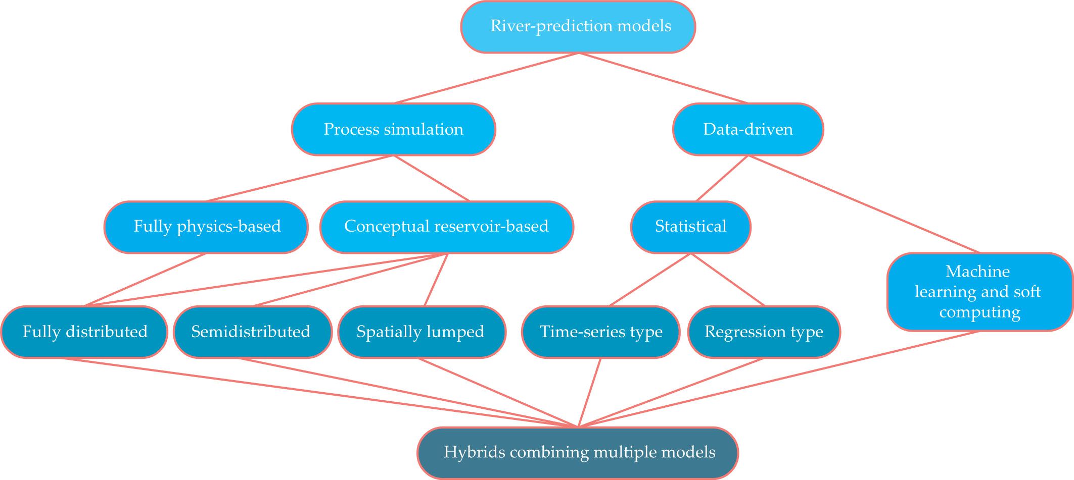
River-prediction models fall broadly into two categories. Process-simulation models aim to be explicitly physics-based and are further classified by their rigor, their level of spatial resolution, and the geophysical and biophysical processes they include. Data-driven models use pattern-detection algorithms to implicitly capture the physics of river runoff generation. They relate predictors to outputs using some form of input–output mapping and are further categorized by their use of classical statistics or artificial intelligence. There is much overlap among the modeling types, and there are many opportunities to combine them.
The Navier–Stokes and continuity equations fundamentally govern fluid transport. To our knowledge, the complete nonlinear equations have never been directly implemented for watershed hydrologic modeling. And for good reason: They’re notoriously difficult to solve numerically, which makes them impractical to implement at the spatial and temporal resolutions and scales typically required. However, with exascale computing on the horizon, applying the full equations may be an idea worth exploring. 4
In 1969 Allan Freeze and Richard Harlan put forward what is widely considered to be the gold standard in hydrologic modeling.
5
Derived from the full Navier–Stokes equations under simplifying assumptions, their physics-oriented approach depicts and predicts nature through a system of coupled partial differential equations that represent water fluxes through landscape elements. (See box
The gold standard
The classical physics-based approach to representing water flows in and across landscapes was first outlined in 1969 by Allan Freeze and Richard Harlan. 5 Their model is built primarily around four coupled partial differential equations. Below are the equations in Freeze and Harlan’s original notation. Today’s models often use more modern formulations, driven in part by advances in computational technology.
The first key element is the Richards equation, which governs water movement in the vadose zone, an unsaturated area above the groundwater table. In their paper, Freeze and Harlan reported that numerical solutions to the three-dimensional Richards equation were not yet possible. They therefore focused on a one-dimensional simplification that only predicted the vertical infiltration of rainfall or snowmelt into the soil:
A less detailed yet widely used hydrologic model approximates water flow using the conceptual linear reservoir assumption. Under that assumption, a watershed’s natural water-storage mechanisms—lakes, wetlands, soil moisture, aquifers, and so forth—act as a de facto reservoir whose output rate depends on how full it is. Combining that with continuity gives the linear reservoir model for river prediction:
A similar but more straightforward treatment considers only continuity without explicitly including the linear reservoir assumption. In such a model, changes in a basin’s water storage are equal to the difference between inputs, like rainfall and snowmelt, and outputs, like evapotranspiration and streamflow. Such water-balance models can be implemented using simple spreadsheet calculations and are sometimes used for practical water-planning tasks. They can also serve as frameworks for building intricate suites of interlinked submodels that represent various additional processes.
The concepts discussed so far represent only two things: the dynamics of water movement across and through the ground and the river basin’s overall water balance. Those elements form the core of any mechanistic river-prediction model. But a river and its watershed can have many different components, such as trees, buildings, swamps, and ice fields. In practice, therefore, most process-simulation models are modular; in addition to their core, they usually integrate several submodels representing environmental factors that can affect streamflow.
Like the cores, submodels vary in their approaches and level of detail. They might represent transpiration by forests and crops, evaporation from lakes and the soil surface, snowpack accumulation and melt, or ice melt from mountain glaciers, which is distinct from seasonal snowmelt. They can also account for near-surface hydrometeorological dynamics, like the dependence of precipitation’s phase on temperature and elevation, which can vary dramatically in rugged mountain watersheds. An estimate of
Models can also account for modifications of natural processes. Capturing land-use changes, such as certain forestry practices that reduce the tree canopy or urbanization of agricultural lands that increases impermeable area, can help predict corresponding shifts in evapotranspiration, snow dynamics, and infiltration. Those shifts can influence river flows by, for example, increasing flood frequency and severity.
An important attribute of any process simulation model is its degree of spatial distribution. A fully distributed model divides the watershed into a grid pattern to accommodate heterogeneity in watershed processes; it can account for details like a thunderstorm only producing rainfall in one part of the watershed. At the other end of the spectrum, a spatially lumped model is a parsimonious approach that treats the watershed upstream of the point of interest as a single homogeneous unit. The intermediate option is a semidistributed model that divides the watershed broadly by spatial proximity or elevation. Some version of either the conceptual linear reservoir or the water-balance method is typically used regardless of a model’s degree of spatial distribution. However, fully distributed models occasionally implement the gold-standard approach, which typically requires a finite-difference solution that leads naturally to a grid-based division of the watershed.
Cyborg hydrologists
Unlike process-simulation models, data-analytics approaches to river prediction view each watershed as a dynamical filter with input and output signals such as rainfall and streamflow. The model’s job is to implicitly capture watershed processes in a transfer function that empirically maps the inputs to the outputs. Such top-down data-driven prediction methods use both statistical and machine-learning techniques, and they serve as a powerful and flexible complement to bottom-up mechanistic models.
Linear Gaussian statistical models have long been used for river prediction. For instance, the 1960s-era Thomas–Fiering model for short-term river forecasting applied standard linear time-series procedures, which are widely used across the natural and social sciences to make predictions from memory-rich datasets. (In fact, Harold Edwin Hurst and Benoit Mandelbrot’s discovery of long-term memory in time series originated from their studies of Nile River flows. Since then, fractal dynamics and 1/f noise in hydrologic data have continued to attract physicists’ attention. 8 ) A more modern example of applying linear Gaussian statistics to river prediction is a probabilistic extension of principal component regression. Originally adapted to water-supply forecasting (WSF) by the US Department of Agriculture, it is commonly used by government agencies and hydroelectric utilities across the western US and Canada to predict seasonal snowmelt volume. 9
Machine learning is a branch of artificial intelligence (AI) that uses algorithms to detect patterns in data and then uses those patterns to make predictions. One of us (Gupta) helped lead the charge 25 years ago to apply machine learning to hydrology;
10
that approach is now coming back in a big way as AI permeates the everyday world. (For more on applying AI to river prediction, see box
Applying artificial intelligence to river prediction
River forecasters were early adopters of machine learning. In the mid 1990s, they began publishing papers that applied artificial neural networks to flood forecasting. Although that research continued, practical applications—particularly to operational forecasts—were few. Roadblocks included an apparent lack of interpretability, an unproven track record, and the deterministic nature of most artificial intelligence (AI) forecasts. However, the use of AI is now becoming routine. Machine-learning algorithms are more accessible, and methods are available for making probabilistic predictions and facilitating the integration of experiential knowledge into machine-learning models. Views are therefore changing toward using AI for practical river-prediction applications.

A hybrid prediction system was recently operationally tested by a flood-forecasting agency in the Pacific Northwest. 18 Several neural-network river-prediction models formed an ensemble; each represented a slightly different geophysical conceptualization of the dominant flood-generating mechanisms in the mountain watershed, which received precipitation as both rain and snow. Each of the neural networks was driven in turn by an ensemble of downscaled and bias-corrected numerical weather predictions from the North American Ensemble Forecast System, a joint project of the US, Canadian, and Mexican national weather services, and by observational data on antecedent streamflow and snowpack conditions. The resulting Monte Carlo super-ensemble, run with a one-day timestep, enabled probabilistic forecasts, including the likelihood of the river topping its banks during the next three days. (Figure adapted from refs. and .)
Current R&D on machine learning for river prediction is bridging the gap between academic research and live operational forecasting systems. Hybrid solutions blend AI with specific technical and institutional requirements around river prediction, including ease of use and alignment with existing knowledge of the physical processes governing river flow. 4 For instance, one of us (Fleming) is currently retrofitting the US Department of Agriculture’s proven WSF model with a physics-constrained AI metasystem that integrates automated machine learning. 11
Data-driven models can easily test the effects of integrating new, potentially helpful information with established predictors. If an update is useful, it can quickly be deployed. For example, El Niño events can cause drier, warmer winters, lower snowpack, and reduced river-flow volumes in the Pacific Northwest; they tend to have the opposite effect in the US Southwest. Climatologists routinely summarize ocean temperature data indicative of such events in compact metrics like the Niño 3.4 index. Hydrologists can easily combine those indices with other predictor variables in a regression- or AI-based WSF model to improve its accuracy. Such practices are common in operational forecasting. However, climate science evolves rapidly, and data-driven models also make it simple to test the river-prediction value of emerging information. They are therefore crucial tools for ongoing hydroclimatic research. 12
Modeling chains
Watershed hydrology is one component of a larger environmental framework, so multiple models are sometimes linked for a more comprehensive view. Gleaning inputs for river prediction models from the outputs of numerical weather-prediction models is a common practice. That chain forms the basis for operational flood forecasting, which provides crucial information for emergency management and dam safety; it facilitates decision-making around whether to issue evacuation notices or preemptively spill water from a reservoir. Government agencies and dam operators generate and use such information daily.
Outputs from watershed hydrology models can also be inputs to river-hydraulics models for mapping flood inundation and propagation. Those models predict where floodwaters will go and how far they’ll reach. Their results are used for emergency planning, setting home insurance rates, and predicting floods in large rivers like the Mississippi, where flood waves from storms far upstream can take days to propagate downstream. Hydraulics models also inform physical habitat assessments; fish like certain kinds of flow patterns, so information about water flow can help protect and restore their habitat.
Basin-scale river-hydrology models coupled with numerical groundwater models can predict the details of river–aquifer interactions. Understanding those relationships has been important for addressing interstate water conflicts like a recent US Supreme Court case between Texas and New Mexico, which was based in part on the effects of groundwater extraction and surface water–groundwater interactions in the Rio Grande basin.
Model chains are also used to assess possible climate change implications for rivers. Outputs from global climate models can be used to drive river predictions; however, the outputs must first be downscaled and bias-corrected to adjust for systematic errors and to provide information about meteorological forcing at appropriate spatial and temporal scales. Climate change may also induce other environmental shifts, such as vegetation changes or glacier recession, that can have hydrologic implications. In those cases, a modeling chain would require intermediate steps to quantify such land-cover changes so they can be represented in the watershed model. Normally, there is no dynamic coupling within a chain; it is a one-way pipeline of offline models run sequentially by different research groups.
Complexity, selection, and ensembles
Many kinds of data are potentially relevant for river prediction. They include land surface characterization, such as maps of vegetation cover and impervious surface area; weather metrics, such as temperature, precipitation, wind speed, and solar radiation; digital elevation models and river network representations; and maps of hydrogeologic characteristics, such as soil types. Sources for those data include long-term environmental monitoring stations, airborne and satellite remote sensing (see figure
Figure 3.

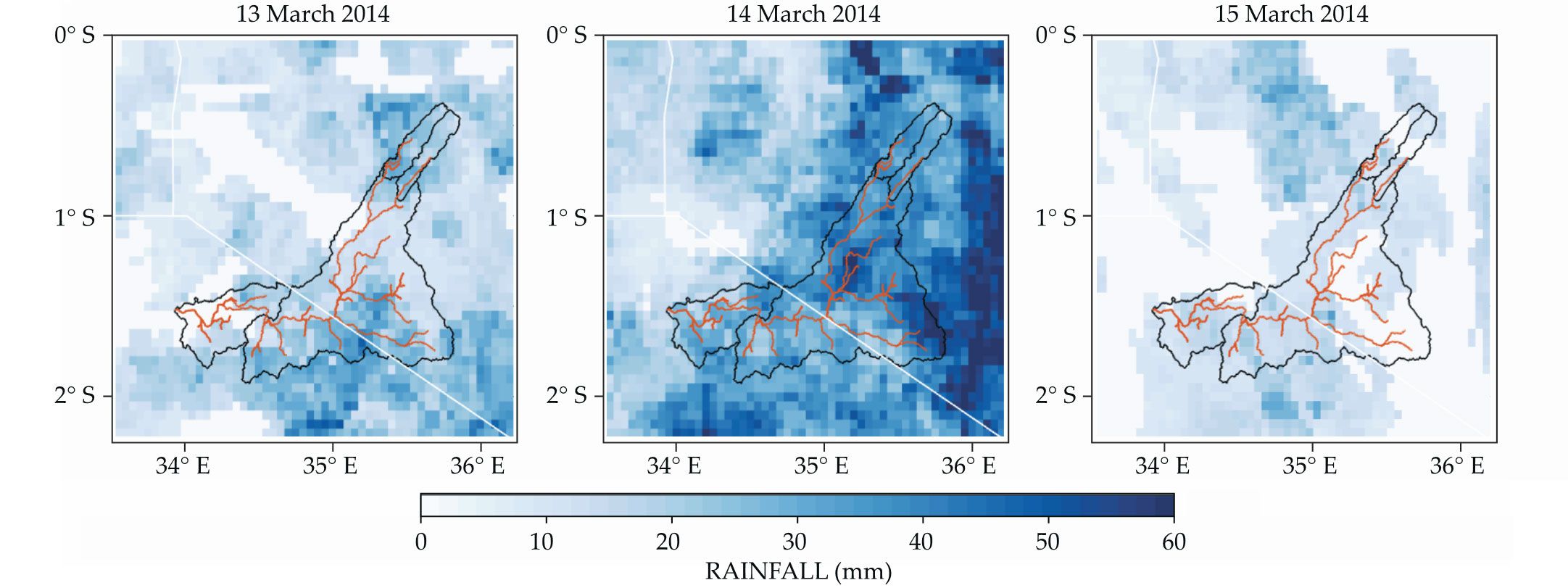
Rainfall in the Mara River basin is tracked by satellite and ground-based measurements and incorporated into the Climate Hazards Group Infrared Precipitation with Stations (CHIRPS) dataset for the region. These maps show daily CHIRPS precipitation; black, orange, and white lines denote, respectively, the watershed boundary, stream network, and Kenya-Tanzania-Uganda borders. Tirthankar Roy and colleagues at the University of Arizona (including one of us, Gupta) combined several satellite-based precipitation products, including CHIRPS, with an ensemble of hydrologic models to provide real-time probabilistic streamflow monitoring and forecasting for the Mara River.
Model choice is less about pros and cons and more about picking the right tool for the job. But that can be challenging. One overarching theme to river prediction models is that there are many, and they’re diverse. Broadly speaking, physics-oriented models are great for testing our hydrologic knowledge because they use explicit representations of specific processes. Their virtual watersheds can also directly simulate predictive scenarios around climate change, urbanization, wildfire, and other long-term environmental shifts. Data-driven models, on the other hand, cost far less to build and run. They also tend to give more accurate short-term operational forecasts of flooding and water supply with more reliable quantitative estimates of predictive uncertainty.
Other selection criteria for a model are whether it represents all pertinent processes; whether it captures the problem’s time and space scales; and whether uncertainty assessment is required. Pragmatic issues also arise, such as reliability, run time, implementation and operating costs, and stakeholder buy-in. New modular, customizable frameworks allow users to choose components. For hydrology, as in many other fields, the best predictive model is often an ensemble.
The value of predictability
River prediction is a high-stakes game, and the stakes are only getting higher. Even modest, incremental improvements in WSF accuracy can contribute additional public value of more than $100 million annually for a single river basin. 13 The accuracy and lead times of flood forecasts are also becoming ever more crucial: Flood risks are escalating with the increased development of floodplains, more extreme rainfall events under climate change, and urbanization-induced losses in the landscape’s capacity to absorb rainfall.

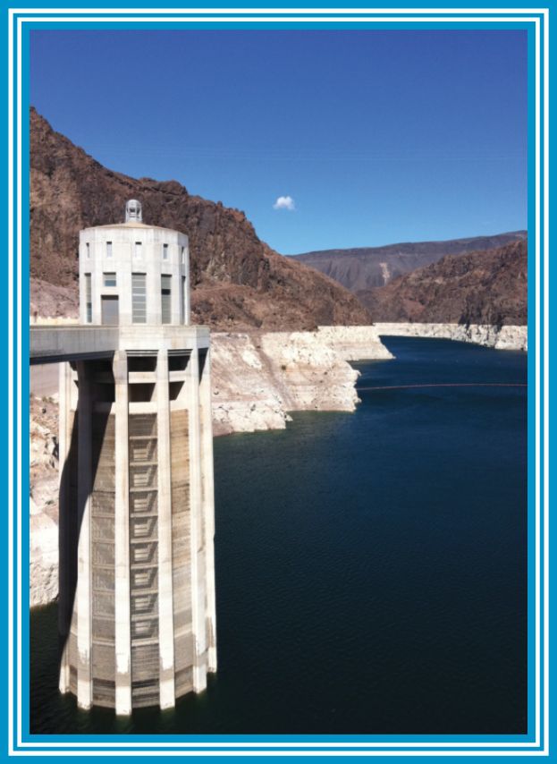
An intake tower at the Hoover Dam. (Photo by Sean Fleming.)
Moreover, two billion people currently live without adequate access to drinking water, and UNESCO expects global water demand to increase by 55% in the next few decades due to population and economic growth. Avoiding lethal and socioeconomically destabilizing global failures to meet basic water-supply needs will require better water-management approaches based on improved understanding and prediction of river dynamics across a range of space and time scales.
Several directions for future work are apparent. 2 , 4 , 14 Predictive skill needs to improve in difficult environments like deserts, alpine watersheds, and dense cities. Renewed attention should be paid to complex systems science, a field that has attracted great interest in statistical mechanics, ecology, and sociophysics. River networks are a classic example of fractal geometry, and chaos theory limits weather’s predictability to an approximately two-week theoretical window. In general, neither of those modern mathematical concepts appears explicitly in river-prediction models; a complex systems approach could incorporate them.
Continuing to capitalize on the data revolution will drive progress in hydrology. Developing novel data types, 15 discovering predictive climatic information, 12 and exploring new analytical directions to support environmental monitoring and prediction 16 all offer opportunities for growth. Substantial forward movement on those fronts will be crucial to managing rivers and water resources in an increasingly uncertain future.
References
1. M. W. Doyle, J. Am. Water Resour. Assoc. 48, 820 (2012). https://doi.org/10.1111/j.1752-1688.2012.00652.x
2. S. W. Fleming, Where the River Flows: Scientific Reflections on Earth’s Waterways, Princeton U. Press (2017).
3. A. T. Wolf, Water Policy 1, 251 (1998). https://doi.org/10.1016/S1366-7017(98)00019-1
4. S. W. Fleming, “Machine learning, soft computing, and complex systems analysis: emerging approaches…,” presentation at the Center for Nonlinear Studies, Los Alamos National Laboratory, 20 August 2018.
5. R. A. Freeze, R. L. Harlan, J. Hydrol. 9, 237 (1969). https://doi.org/10.1016/0022-1694(69)90020-1
6. S. L. Painter et al., Water Resour. Res. 52, 6062 (2016). https://doi.org/10.1002/2015WR018427
7. S. J. Kollet et al., Water Resour. Res. 46, W04201 (2010). https://doi.org/10.1029/2009WR008730
8. V. N. Livina et al., Phys. Rev. E 67, 042101 (2003). https://doi.org/10.1103/PhysRevE.67.042101
9. D. C. Garen, J. Water Resour. Plan. Manag. 118, 654 (1992). https://doi.org/10.1061/(ASCE)0733-9496(1992)118:6(654)
10. K. Hsu, H. V. Gupta, S. Sorooshian, Water Resour. Res. 31, 2517 (1995). https://doi.org/10.1029/95WR01955
11. S. W. Fleming, A. G. Goodbody, IEEE Access 7, 119943 (2019). https://doi.org/10.1109/ACCESS.2019.2936989
12. A. M. Kennedy, D. C. Garen, R. W. Koch, Hydrol. Process. 23, 973 (2009). https://doi.org/10.1002/hyp.7200
13. A. F. Hamlet, D. Huppert, D. P. Lettenmaier, J. Water Resour. Plan. Manag. 128, 91 (2002). https://doi.org/10.1061/(ASCE)0733-9496(2002)128:2(91)
14. M. P. Clark et al., Hydrol. Earth Syst. Sci. 21, 3427 (2017). https://doi.org/10.5194/hess-21-3427-2017
15. T. H. Painter et al., Remote Sens. Environ. 184, 139 (2016). https://doi.org/10.1016/j.rse.2016.06.018
16. M. J. Halverson, S. W. Fleming, Hydrol. Earth Syst. Sci. 19, 3301 (2015). https://doi.org/10.5194/hess-19-3301-2015
17. T. Roy et al., J. Hydroinformatics 19, 911 (2017). https://doi.org/10.2166/hydro.2017.111
18. S. W. Fleming et al., J. Am. Water Resour. Assoc. 51, 502 (2015). https://doi.org/10.1111/jawr.12259
More about the authors
Sean Fleming is an applied R&D technical lead at the US Department of Agriculture’s Natural Resources Conservation Service in Portland, Oregon, and an affiliate faculty member at Oregon State University in Corvallis and the University of British Columbia in Vancouver. Hoshin Gupta is a Regents’ professor in the department of hydrology and atmospheric sciences at the University of Arizona in Tucson.


