The Atmospheric Radiation Measurement Program
DOI: 10.1063/1.1554135
Ten years ago, at the dedication of the first research site of the Department of Energy’s Atmospheric Radiation Measurement (ARM) program, near Lamont, Oklahoma, Will Happer, director of DOE’s Office of Science, compared the nascent facility to Uraniborg, the island observatory built by Tycho Brahe in 16th-century Denmark. That comparison puts the role of ARM climate-research facilities in an interesting perspective. A decade after its creation, ARM is well on the way to providing data essential to climate research and weather prediction in much the same way that Tycho’s observations were essential to the subsequent work of Johannes Kepler.
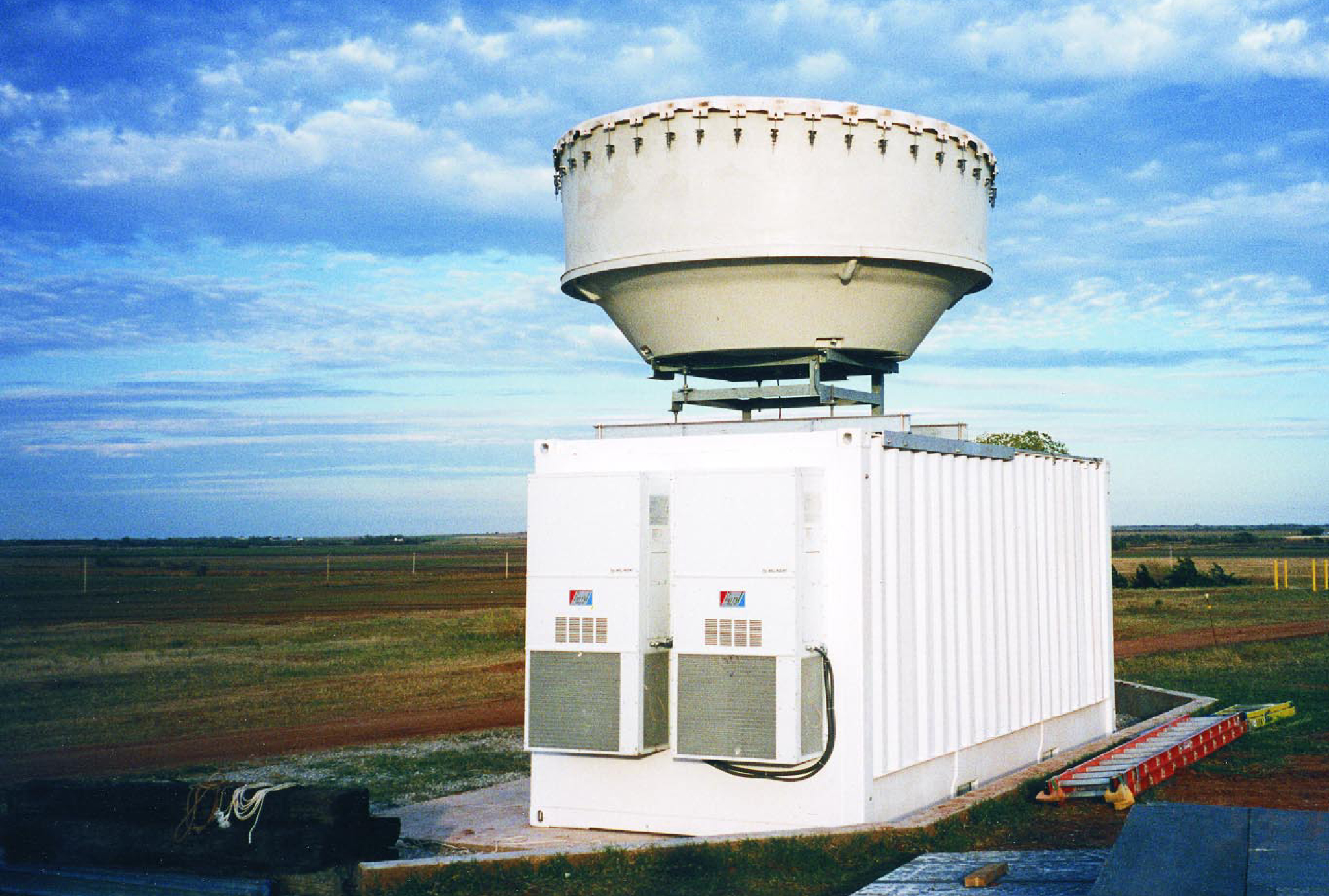
Like Uraniborg, ARM’s central facility at Lamont has become the accumulation site for some of the most sensitive instruments available for its mission (see figure 1). Tycho had collected, in one place, the finest astrometric instruments of his day—four decades before Galileo introduced the astronomical telescope. Ironically, Tycho had too much confidence in his measurements: He maintained that they disproved Copernicus’s heliocentric cosmology, because they showed no discernable stellar parallax. In the end, of course, the quality of Tycho’s observations contributed to the overthrow of his own geocentric cosmology.

Figure 1. Cloud radar system at the central facility of the Atmospheric Radiation Measurement (ARM) program, near Lamont, Oklahoma, probes the extent and composition of clouds over the site at millimeter wavelengths. ARM was created to elucidate the interaction between clouds and radiative fluxes in the atmosphere for the purpose of creating better climate and weather models.
DOE ATMOSPHERIC RADIATION MEASUREMENT PROGRAM
It is unlikely that ARM will motivate anything as profound as the Copernican revolution. But it has already begun to lay the foundation for great improvement of climate models, and it serves as an important test bed for the physics of climate and weather-prediction models.
Clouds and climate models
The scientific motivation for the ARM program arose from a decade of comparisons of different climate models. Those comparisons sought to elucidate the underlying reasons for the substantial and disconcerting differences, from one model to another, in their predictions of climatic responses to such perturbations as the doubling of atmospheric carbon dioxide.
The comparisons produced two important results in the late 1980s. One such undertaking, called the Inter-comparison of Radiation Codes in Climate Models, showed that when radiative transfer through the atmosphere was understood at high spectral resolution, it was possible to create a fast, lower-resolution model appropriate for climate modeling. The low-resolution models were needed because of limitations on computing power and on the availability of sufficient measurements to validate the high-resolution models, especially in the context of complex three-dimensional cloud fields. Other comparisons of climate models suggested that the predicted sensitivity of global temperature to greenhouse gases was directly related to how the models treated the interaction of clouds with radiation. In particular, a study led by Robert Cess (Stony Brook University), 1 compared the response of a variety of atmospheric climate models to changes in sea-surface temperature and showed that model responses varied over nearly an order of magnitude. The different responses were due almost entirely to differences in the treatment of clouds and their impact on solar and thermal infrared radiation.
In 1990, the treatment of clouds in climate models was identified as the highest-priority research topic in the newly formed United States Global Change Research Program. ARM was created to meet this challenge. The central facility at Lamont sits in the middle of the 140 000-km2 ARM Southern Great Plains site, which is dotted with more than a dozen instrumented satellite facilities stretching up into Kansas (see figure 2). The research at the Southern Great Plains site, and at smaller ARM facilities around the world, has led to the refinement of state-of-the-art meteorological instruments and of the techniques that employ them. Specific accomplishments include advances in cloud radars and high-resolution spectroscopy, the first continuously operating Raman lidar system for profiling water vapor, and the use of unmanned aerospace vehicles for atmospheric observations. (Lidar is much like radar, except that it observes the reflection of light—visible, infrared, and ultraviolet—instead of radio waves. Inelastic Raman scattering of the laser light can be used to identify molecular species.) Such instruments have given us an invaluable archive of observations for understanding the propagation of radiation through the atmosphere, and the effect of clouds on that propagation.

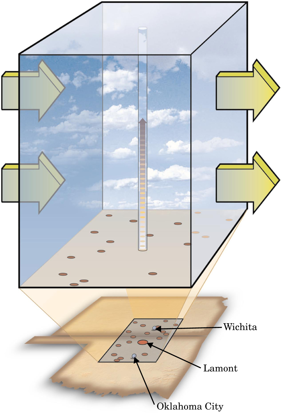
Figure 2. The ARM Southern Great Plains site surrounds the Lamont, Oklahoma, facility with 17 satellite stations deployed throughout the 140 000-km2 site in Oklahoma and Kansas. The atmospheric cube covering the site represents a single-column climate model; the arrows indicate the energy and water transport that determine the column’s lateral boundary conditions. The much narrower column at the center represents radar, lidar, and other instruments probing the clouds in a conceptual “soda straw” over the Lamont facility.
The goal of the ARM program is to increase our understanding of the interaction between clouds and atmospheric radiative fluxes, and then to capture that knowledge in improved climate models. From an observational perspective, the focus is on measuring the solar and thermal infrared radiative fluxes at Earth’s surface, and all of the atmospheric quantities that affect those fluxes.
Even before ARM, scientists had already made such efforts in field campaigns that lasted for a month or two. ARM’s unique innovation was to perform the measurements continuously for a decade or more. Earlier field campaigns had relied heavily on aircraft. But the high cost and limitations of research aircraft restrict long-term continuous measurement to instruments that sample the atmosphere remotely from the ground. Remote sensing of the atmosphere, whether from the ground or from satellites, depends primarily on spectrally resolved radiation measurements.
ARM remote sensing involves both passive and active instruments. Passive ground-based remote sensing relies on measurements of not only solar radiation transmitted through the atmosphere, but also of thermal radiation—both infrared and microwave—emitted by the atmosphere. Similarly, satellite remote sensing measures thermal radiation from the ground and the atmosphere, and also reflected solar radiation. Because the transmission and emission depend on specific properties of the atmosphere, one can use these passive measurements, particularly when they are made in narrow spectral intervals, to analyze the state of the atmosphere.
Active ground-based remote sensing uses pulsed electromagnetic radiation sources such as lasers and radars to probe atmospheric structure. Measurements of backscattered radiation from lidar or pulsed laser systems provide information on the vertical structure of thin clouds and particle distributions. Millimeter-wave radar systems probe the vertical structure of thin and thick clouds.
Global grids
Large-scale models of the atmosphere, whether for climate studies or weather prediction, consist of coupled sets of differential equations for the atmospheric state variables: pressure, temperature, wind velocity, and water-vapor pressure. These equations are prognostic in the sense that each equation has a time derivative that lets us approximate the future state of the atmosphere from its current state. The equations are solved on a rather coarse spatial grid, typically with horizontal steps on the order of several hundred kilometers, and anywhere from 10 to 40 vertical layers. Still, because the models are global, the total number of grid points is very large. With time steps on the order of a half hour, these models require enormous amounts of computer time.
From the perspective of our concern with clouds, however, the most important issue is something that the prognostic equations of these models cannot compute. Any process that occurs on scales smaller than the grid cell dimensions must be inferred from the predicted state variables in that cell. For example, if the predicted water-vapor pressure in a cell at some time step exceeds the saturation vapor pressure at the predicted cell temperature, we can infer that condensation must occur, which in turn means that clouds must form. The model cannot, however, explicitly represent the clouds. We must, instead, treat them by some statistical parametrization—highly simplified expressions for the actual physical processes, generally involving a set of adjustable parameters. Setting the values of these parameters is done by a combination of theory and observation.
The cloud field produced in a grid box of a global climate model by such parameterization equations is obviously a crude simplification of the real clouds. It cannot capture either the spatial structure at subgrid scale or the associated variability of cloud properties. Therefore, the calculation of radiative transfer through the clouds is also simplified. So the first question that we need to answer is: Given a specified three-dimensional field of cloud properties, can we compute with sufficient accuracy the solar and terrestrial radiative flux transfer and associated atmospheric heating rates through the clouds?
A so-called soda-straw view of the radiative transfer problem provides the conceptual framework for gathering data to answer the question. One imagines an isolated hollow straw, a few kilometers in diameter, vertically spanning the atmosphere from its top to the ground. This kind of conceptual sampling corresponds to the sparse sampling character of the available data. One simply can’t cover the ground densely with expensive measuring facilities.
Solar radiation that hits the top of a straw is either reflected back, transmitted all the way through to the bottom of the straw, or absorbed along its length. In the opposite direction, radiation from Earth’s surface is likewise either reflected, absorbed, or transmitted by the straw. How the radiation hitting a conceptual straw at either end is partitioned among reflection, absorption, and transmission is a function of the atmosphere’s state. The radiatively significant atmospheric constituents are gas molecules, particles, and water in the form of cloud droplets, ice crystals, and precipitation.
The ARM observatory
The Lamont site is the central facility of the ARM observatory. It is designed to sample continuously all the components of the radiation budget at Earth’s surface and all the relevant constituents in the atmosphere above the site. The atmospheric observables include the presence of clouds, their vertical extent, and their radiative properties. The extent of the clouds is measured with active sensors—radar and lidar. But measuring their radiative properties also requires the use of passive sensors.
Beyond the question of our ability to compute radiation through clouds with sufficient accuracy lies a second, more difficult, question: Given the large-scale predicted or measured states of the atmosphere, can we predict the statistical properties of the local cloud fields? In other words, can we make the diagnostic connection between the large-scale atmospheric fields and the subgrid-scale clouds?
The ARM program has two modeling approaches to that problem. The first we call single-column modeling. A conceptual column is much like a soda straw, except that its diameter, corresponding to a grid spacing, is several hundred kilometers wide. Because different altitudes in the atmosphere couple rapidly with each other through vertical convection and boundary-layer processes, most model cloud parameterizations are designed to treat each vertical column as an almost independent entity. Horizontal transport across the column’s lateral boundary, by contrast, occurs in such models only by advection, that is, by large-scale horizontal wind.
Thus we can imagine isolating a single column of the larger dynamical model, if we can supply the boundary advection terms. The physical parameterizations in such a single-column model run largely as they would in the full model, because they depend only on the vertical coupling and the values of the local variables. To run a single-column model, one must specify the advective terms at the column’s boundaries and the vertical surface fluxes at its top and base on a scale consistent with the grid size of a global climate model (see figure 2).
A second approach to the problem of predicting the statistical properties of the local cloud fields involves the use of cloud-resolving models. Running at small spatial scales of a kilometer or less, these models seek to resolve actual cloud processes and the coupling between clouds and atmospheric dynamics. To the extent that such models can simulate actual atmospheric events, their output can be used to develop parameterizations for models with coarser resolution. Running a cloud-resolving model requires putting in essentially the same set of boundary conditions—horizontal advective fluxes and radiative fluxes at the top and bottom of the atmosphere—that one needs for a single-column model.
Evaluating the results of experiments that test single-column and cloud-resolving models requires knowing the 3D cloud structure on a scale of a hundred kilometers. To adequately determine the perturbing atmospheric fields, the ARM observatory has had to expand to a much greater range of measurements than we can make at just the Lamont central facility. Performing all the measurements needed for the soda-straw model is daunting. On page 41, the
Measurements Required for Soda-Straw Climate Models
| Atmospheric Variables | Instrument Types |
|---|---|
| Surface radiation budget | Broadband solar and IR radiometers |
| Shadow-band radiometer (narrow spectral bands) | |
| Spectrometer (400–3000 nm) | |
| Interferometer (3–20 µm) | |
| Atmospheric temperature profile | Balloon-borne sounding probes |
| Interferometer (3–20 µm) | |
| Water-vapor profile | Narrow-band microwave radiometer (24, 31 GHz) |
| Interferometer (3–20 µm) | |
| Balloon-borne sounding probes | |
| Particle optical depth | Narrow-band sun photometer |
| Shadow-band radiometer (narrow spectral bands) | |
| Cloud location | Millimeter radar (35 GHz) |
| Lidar (532 nm) | |
| Cloud properties | Millimeter radar (35 GHz) |
| Lidar (532 nm) | |
| Radiometers (solar, IR, microwave) |
To characterize the atmosphere and boundary fluxes on the spatial scales needed for the single-column and cloud-resolving model simulations, we require additional measurements at external sites scattered throughout the Southern Great Plains site and on its borders. We would like to duplicate the entire instrument suite at each of these external sites, but that’s not possible. So our external sites measure only surface energy fluxes, standard weather parameters, and some integrated column quantities. When data from the satellite facilities are included, the archiving rate grows to 3.7 GB per day. This volume is the aggregate of almost 1000 individual instruments.
In addition to data from the ARM instruments, the observatory routinely archives voluminous atmospheric data from other sources: remote measurements from satellites, 3D wind measurements from the National Oceanic and Atmospheric Administration’s radar wind-profiler array, and meteorological parameters from weather-forecasting centers. All of these data can be distributed in near real-time to the ARM science team.
In addition to its longer-term undertakings, the ARM observatory provides opportunities for special intensive operational periods (IOPs), directed at specific science problems. For example, IOPs have been directed at understanding the accuracy of routine atmospheric measurements, and at specific cloud problems such as anomalous absorption of solar radiation. The IOPs have generally required expanded surface instrumentation and aircraft or unmanned aerospace vehicles. For many of the IOP efforts, the availability of the continuous ARM measurements is a unique asset.
The ARM observatory now ranges far beyond the Southern Great Plains site. In the late 1990s, ARM began observations on several islands in the tropical western Pacific. Continuous arctic observations started at Barrow, Alaska in 1998. These far-flung smaller facilities focus on the soda-straw approach. Most recently, ARM has installed a site at Darwin, in tropical northern Australia, in partnership with the Australian Bureau of Meteorology.
Science at ARM
Here we briefly summarize three different examples of atmospheric radiation science problems that have been addressed by the ARM observatory:
-
▸ Many investigators use ARM measurements to study issues of radiative heat transfer. For example, the atmospheric infrared window at wavelengths from 8 to 12 µm plays a very important role in regulating the loss of thermal energy from our planet. The peak blackbody emission at typical Earth surface temperatures falls in this spectral window. But spectral line and continuum absorption by water vapor render this window only partially transparent. Therefore, the magnitude of radiant cooling depends critically on the H2O absorption coefficients. In the absence of an adequate theory from which the continuum coefficients can be computed, our treatment of this important spectral feature relies on a combination of limited theory and empirical fits.
The problem cannot easily be addressed in the confines of a laboratory. Integrated water-vapor column densities of vertical paths through the entire atmosphere typically range from a fraction of a gram per cm2 to about 7 g/cm2. Such column densities are very difficult to duplicate within the confines of a laboratory cell. Being much shorter than the height of the atmosphere, the laboratory cell would necessitate a correspondingly greater vapor density. But then the vapor would condense, unless it was heated. The requisite high temperature and pressure, however, would not adequately simulate atmospheric conditions. But the ARM observatory can acquire the necessary data simply by waiting for a cloudless sky within the soda straw. (One needs to avoid clouds because they are very efficient emitters of thermal radiation.)
We have carried out such measurements at the central Lamont site using an interferometer that measures atmospheric emission from 5 to 20 µm. These data, in conjunction with data acquired in the tropical western Pacific, have been used to provide an improved model of continuum water-vapor absorption. 2 Figure 3 compares the measured infrared radiance against computations of the radiance with the improved model and an earlier model. The excellent agreement of the new model with the measurements indicates that our understanding of the water-vapor continuum and line absorption has improved substantially over the course of the ARM program.

Figure 3. Thermal radiation by the atmosphere, plotted (top panel) against reciprocal wavelength, shows the atmospheric window between 8 and 12 µm that lets thermal radiation from Earth’s surface escape into space. The atmospheric absorption is measured by an infrared interferometer on the ground that looks up at the zenith on a cloudless Oklahoma day. The trough, showing weak continuum water-vapor emission, is filled with discrete H2O lines and hemmed in at its long-wavelength end by strong CO2 absorption. The bottom panel shows the observed minus the calculated radiance both for a new model
(Courtesy of David Turner, University of Wisconsin.)

-
▸ Our second example deals with radiation from the Sun rather than from the planet’s surface. This is the so-called anomalous absorption problem. For many years, attempts to measure solar absorption in clouds have produced values that exceed computed expectations. The differences were typically less than 10 or 15%, and they could plausibly be explained away by measurement uncertainties, cloud inhomogeneities, or other minor effects. But some authors have argued that the anomaly may be as high as 50%. 3 And such large discrepancies, implying the action of unknown processes in the atmosphere, would have serious implications for our understanding of the role of radiative transfer in the climate system.
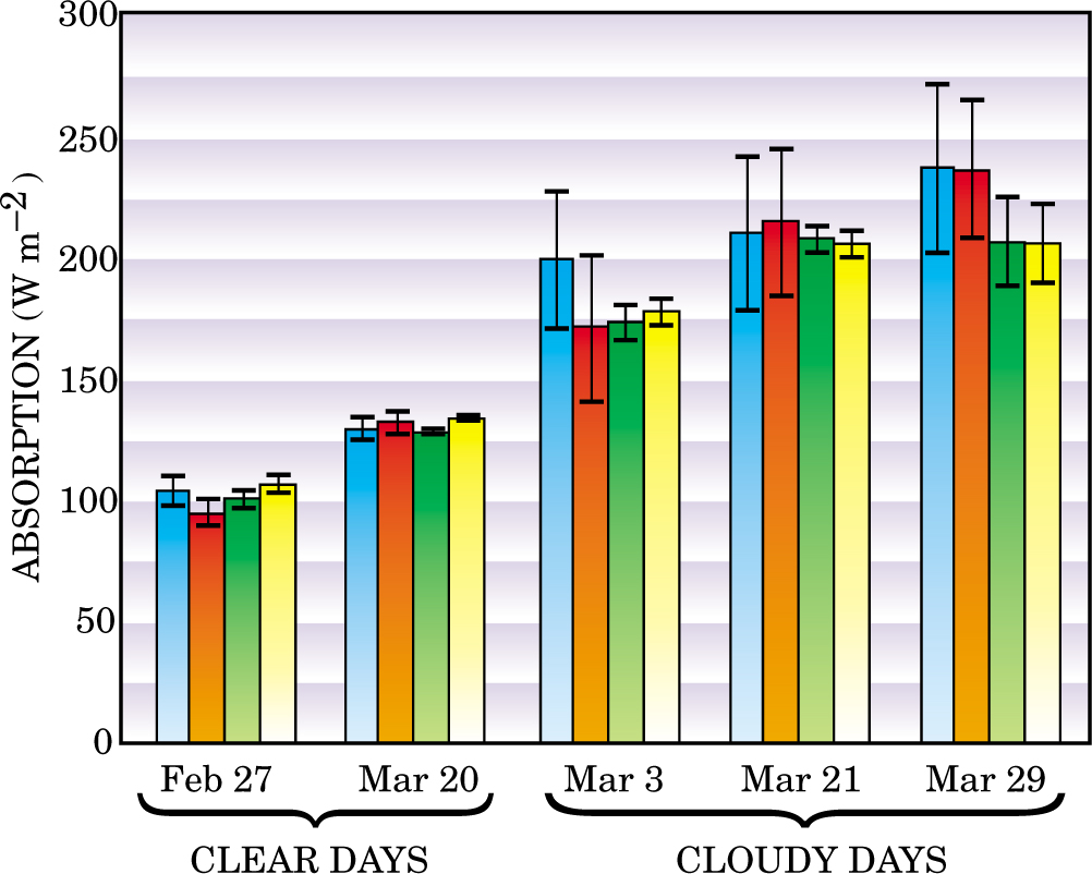
Two years ago, after several inconsistent experimental results from ARM and elsewhere, we sponsored a new enhanced-shortwave experiment that would, we hoped, finally lead to consensus. The new experiment made good use of ARM’s central facility, where continuous measurements of the upward and downward radiative fluxes were available, as were measurements of atmospheric and cloud properties. We added three sets of broadband solar radiometers mounted on an aircraft, which was flown over the site and above stratiform clouds at an altitude of 7 km. Model calculations of solar radiation require input profiles of temperature and molecular gas absorbers, particulate composition and distribution, cloud location, water droplet distributions, and surface spectral reflectivity. Routine ARM measurements provided most of these profiles with high temporal resolution. The solar absorption on clear days and cloudy days was obtained from aircraft and ground measurements.
The results, shown in figure 4, suggest that, although the measured absorption does exceed the computed expectation in some cases, the differences are small enough to be explained by reasonable extensions of our current understanding of atmospheric physics. In essence, then, the troubling anomalous-absorption problem has largely gone away.

Figure 4. Solar absorption by a column of air extending from the ground up to 7 km was measured by comparing ground and aircraft measurements at the Southern Great Plains site on two clear days and three cloudy days in 2002. The blue and red columns show measurements with two different radiometer sets, and the green and yellow columns show the predictions of two different models. The differences between these recent measurements and the predictions are reassuringly small.
(Adapted from ref. 7.)
-
▸ The third example involves cirrus clouds. The ARM observatory compiles statistical distributions of these very high clouds, which are composed of ice crystals. Found in the upper troposphere at altitudes between 5 and 16 km, these clouds are typically less optically thick than clouds at lower altitudes, whose liquid water droplets are generally smaller than the cirrus ice crystals. Therefore the cirrus clouds reflect less solar radiation than do the water clouds. On the other hand, even tenuous cirrus clouds absorb significant amounts of thermal infrared radiation emitted by the ground and the lower atmosphere. Thus, these high cloud layers play an important role in increasing the greenhouse capacity of Earth’s climate system.
But cirrus clouds are notoriously difficult to model, because the processes that create them are complex and incompletely understood. Their altitude makes direct observation from aircraft problematic. Laboratory experiments on ice growth cannot adequately capture the complexity of cirrus cloud formation in the free atmosphere. Remote sensing techniques at the ARM observatory, on the other hand, offer the opportunity to greatly increase our understanding of cirrus clouds.
ARM’s remote-sensing techniques combine millimeter-wave cloud radar with thermal infrared interferometry. The radar directly measures the height and extent of the cirrus clouds, and the magnitude of the back-scattered radar signal depends on the total ice mass and the distribution of particle sizes. The downward radiance measured by the infrared interferometer is a combination of thermal emission by atmospheric water vapor and by the cloud ice mass. From the radar and infrared data, together with balloon measurements of atmospheric temperature and moisture, one can deduce the emission from the clouds alone.
Atmospheric ice particles rarely exhibit the pristine hexagonal shapes predicted by classical studies of slow ice growth. They are most often quite irregularly shaped. The effective diameters of the ice particles are typically less than 100 µm, which puts them in the small-particle scattering limit for the radar. The millimeter-wave radar is most sensitive to the largest ice particles in the size distribution. But even the smaller particles are large compared to the 10-µm wavelength of the atmospheric infrared emission we sample. We take advantage of these different instrumental sensitivities to determine the integrated column ice mass and the mean ice-particle size. 4
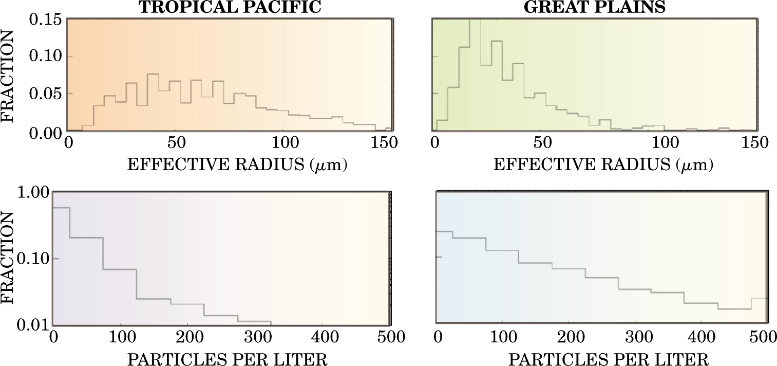
Figure 5 shows the concentration and size distribution of ice crystals in cirrus clouds as measured by ARM with this combination of radar and IR interferometry at the Southern Great Plains site and in the tropical Pacific. At the tropical site, the average height of the cirrus layers was 13 km. That’s 4 km higher than at the US site. The crystals are larger in the tropics, but there are fewer of them, per unit cloud volume, than at the midlatitude site. These differences probably reflect different cloud-forming mechanisms at different latitudes. Because we make simultaneous measurements of atmospheric properties, we can relate the cirrus properties to details of the atmospheric state. These empirical relationships form the basis for parameterizations to be used in climate models.

Figure 5. Ice crystal distributions in cirrus clouds measured by ARM in the tropical Pacific and at the Southern Great Plains site. A combination of millimeter-wave radar, ground-based infrared interferometry, and balloon measurements yields effective particle radii (top panels) and number density (bottom). The ice particles in the higher-lying tropical clouds are typically larger, but there are fewer of them per unit cloud volume.
(Courtesy of Gerald Mace, University of Utah.)
These three examples illustrate that, given a detailed description of the properties of an atmospheric soda straw, we can now generally compute its radiation transport to the accuracy required for atmospheric modeling. There remain, of course, unresolved issues related to the modeling of complex cloud geometries.
Parameterizing clouds
In the past, atmospheric observations at midlatitudes were insufficient for creating the single-column and cloud-resolving models. There were too few observations, they had rather large measurement errors, and they did not capture small-scale motions. Analyses based only on such limited observations could not provide the reliable descriptions of the large-scale atmosphere one needs for establishing the lateral boundary conditions—the so-called forcing fields—in such models.
ARM’s solution to this difficulty is a hybrid approach. One begins with an analysis of the current atmospheric state, available from the National Weather Service. Then one interpolates smoothly into this analysis all the available data from the discrete ARM sites. Finally, one carries out a variational-calculus computation that imposes the constraints of mass and energy conservation on the interpolated data fields. 5 ARM can now provide these computed fields continually to the modelers. That lets them compare the predictions of the different models with each other and with the actual atmospheric observations.
Consider, for example, a simulation for a two-week period in the summer of 1995 of the atmosphere above the entire Southern Great Plains site. Eleven different single-column models and one cloud-resolving model were run for this period, all updated every few hours with the same forcing fields measured at the sides of the column, at the ground, and at the top of the atmosphere. 6 figure 6 shows the time variation of temperature, averaged horizontally over the entire site and vertically from the ground almost to the top of the atmosphere, as predicted by the different models, and as actually observed.

Figure 6. Comparing various climate model calculations (colored curves) with the measured mean atmospheric temperature (black curve) over the ARM Southern Great Plains site for two weeks in the summer of 1995. Except for one cloud-resolving-model curve (labeled), all the other colored curves are calculated from single-column models. All the models were fed every three hours with the same updated boundary conditions measured at the sides, top, and bottom of the column. Still, with increasing time, the model curves drift farther and farther from the measured initial temperature and from each other.
(Adapted from ref. 6.)
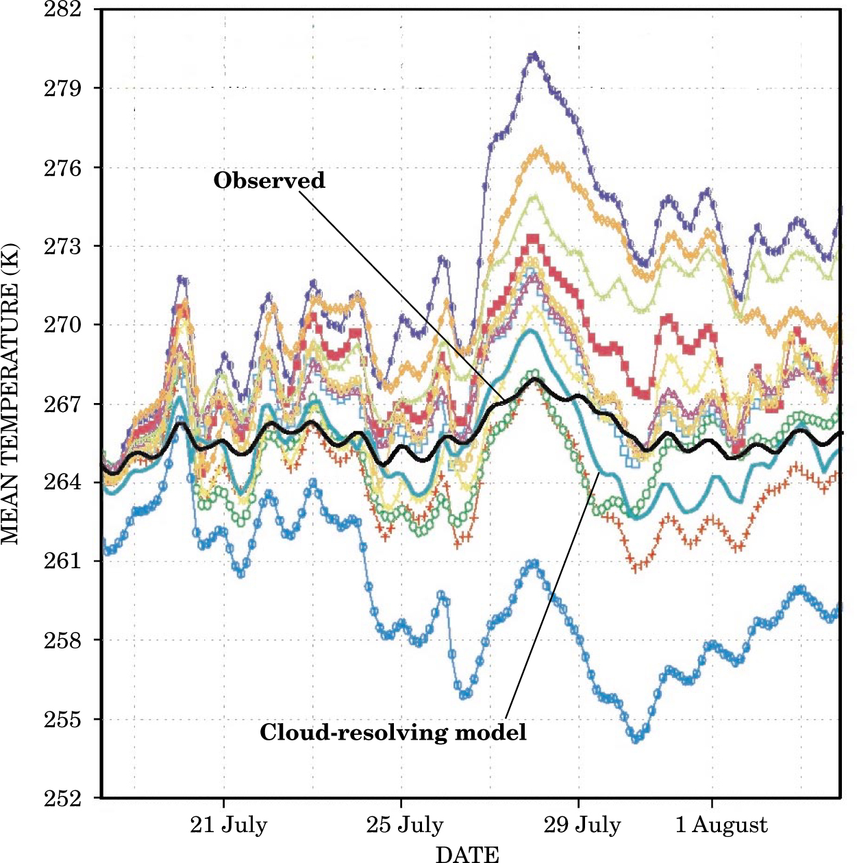
Note that the model predictions increasingly drift away from the measured temperature as time passes. The drifts are large, and they differ significantly from model to model. The fact that all the models show similar excessive excursions at certain times (20 July, for example) is indicative of substantial errors in the specified forcing fields at those times. By separating the errors into those common to all models and those that are model specific, we begin to isolate the processes within specific models that are not well modeled. And then we undertake to modify the parameterizations accordingly.
Lessons and prospects
The ARM atmospheric observatory celebrated the 10th anniversary of its conception in 2000. The deployment of instruments at the central facility began in 1992 and was completed with the installation of the millimeter-wave radar system four years later. Our experience has turned pioneering remote-sensing systems from intensively manned research devices into routine, semiautonomous instruments.
As the quality of our data has improved over time, the focus of our research has shifted. Much of the initial effort was on instrument development and basic radiative-transfer theory. This gradually gave way to studies of atmospheric processes. Now we have moved toward a greater emphasis on comparing models with observations and evaluating parameterizations.
Along the way, we have encountered surprises. An intriguing development is the close cooperation that has evolved between ARM and operational centers for weather forecasting. The forecasting centers have found the ARM data to be extremely helpful for evaluating and improving their models. And they, in turn, have supplied research support and ideas to the ARM community. Quite generally, the use of the ARM observatory by other programs has greatly exceeded our expectations.
The ARM observatory has become an integral component of international collaborations and of US government research programs sponsored by agencies such as NASA and the National Oceanic and Atmospheric Administration. Although the Southern Great Plains site remains our premier facility, data from the remote ARM sites in Alaska and the Pacific are widely used to study polar and tropical climates. Japan, Australia, and several countries in Europe have expressed interest in creating observatories like ARM.
This world-wide interest bodes well for the future of ground-based remote sensing for climate modeling and weather forecasting. Along with continued observation at the existing ARM facilities, we also hope to build a mobile facility that would extend the kind of measurements our remote fixed sites now perform to any place on Earth for periods up to 18 months.
References
1. R. D. Cess et al., J. Geophys. Res. 95, 16601 (1990) https://doi.org/10.1029/JD095iD10p16601 .
2. E. R. Westwater et al., Bull. Am. Meteorol. Soc. 80, 257 (1999) https://doi.org/10.1175/1520-0477(1999)080<0257:GBRSOD>2.0.CO;2
D. C. Tobin et al., J. Geophys. Res., 104, 2081 (1999) https://doi.org/10.1029/1998JD200057 .3. R. D. Cess et al., Science 267, 496 (1995) https://doi.org/10.1126/science.267.5197.496
P. Pilewkie, F. Valero, Science 267, 1626 (1995) https://doi.org/10.1126/science.267.5204.1626 .4. G. Mace, T. Ackerman, P. Minnis, D. Young, J. Geophys. Res. 103, 23207 (1998) https://doi.org/10.1029/98JD02117
G. Mace, K. Sassen, S. Kinne, T. Ackerman, Geophys. Res. Lett. 25, 1133 (1998) https://doi.org/10.1029/98GL00232
G. Mace, E. Clothiaux, T. Ackerman, J. Climate. 14, 2185 (2001) https://doi.org/10.1175/1520-0442(2001)014<2185:TCCOCC>2.0.CO;2 .5. M. Zhang, J. Lin, R. Cederwall, J. Yio, S. Xie, Mon. Weather Rev. 129, 295 (2001) https://doi.org/10.1175/1520-0493(2001)129<0295:OAOAID>2.0.CO;2 .
6. S. Ghan et al., J. Geophys. Res. 105, 2091 (2000) https://doi.org/10.1029/1999JD900971 .
7. T. Ackerman, D, Flynn, R. Marchand, J. Geophys. Res. (in press).
More about the authors
Thomas Ackerman is a Battelle Fellow at the Pacific Northwest National Laboratory in Richland, Washington, and chief scientist of the Department of Energy’s Atmospheric Radiation Measurement program. Gerald Stokes, the program’s previous chief scientist, is now director of the Joint Global Change Research Institute at the University of Maryland, College Park.
Thomas P. Ackerman, Pacific Northwest National Laboratory, Richland, Washington, US .
Gerald M. Stokes, Joint Global Change Research Institute, University of Maryland, College Park, US .


