Spontaneous generation of internal waves

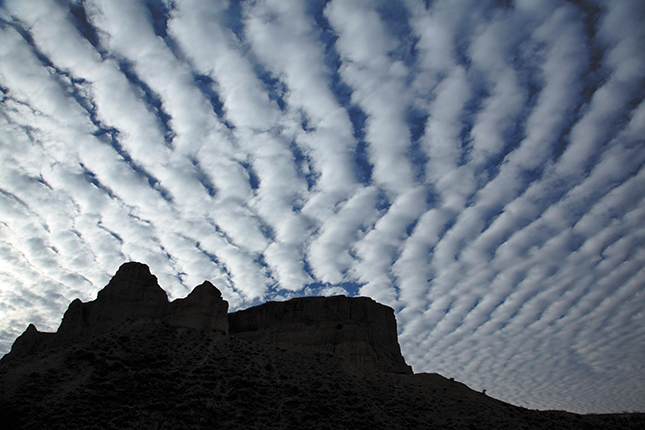
Look up at the sky on a cloudy day, and you often see sets of parallel, equally spaced bands of clouds that are the signature of a type of wave known as an internal wave. Although visible under only the right conditions, internal waves are ubiquitous in both the atmosphere and the ocean. In many dynamical systems, waves release excess energy in a fluid that is displaced from its lowest-energy, balanced state. Internal waves extract and transport energy three-dimensionally before releasing it to large-scale circulation.

Historically, researchers thought that only mechanical forcing or direct thermal displacement of the system from its balanced state could generate internal waves. However, more recent work shows that a spontaneous imbalance of the fluid system can generate or amplify them without any direct forcing. The discovery has led to new perspectives on the role of waves in the circulation of the atmosphere and ocean. (For more on internal waves in planetary atmospheres, see the article by Erdal Yiğit and Alexander S. Medvedev on page 40 of this issue.)

Waves that you see on the surface of an ocean are near cousins of internal waves, and fluid dynamicists call them surface gravity, or just surface, waves. Strong storms generate surface waves, which are periodic oscillations in the height of the water, and they can propagate 10 000 km across entire ocean basins before they break on your local beach. The motion of surface waves is confined to the two-dimensional surface of the ocean. In contrast, internal waves, which storms also generate, propagate three-dimensionally through the ocean’s interior as periodic oscillations in the height of stratified constant-density layers. For some internal waves, the oscillations are a hundred meters or more in amplitude—far larger than surface waves.

All waves have a dispersion relation, which quantifies the relationship between wavelength and frequency in terms of certain physical parameters. The two important parameters for internal waves are the Coriolis frequency and the buoyancy frequency. The Coriolis frequency f is the vertical component of Earth’s rotation vector at a fixed point on its surface and depends on latitude. The value of f sets the minimum frequency for internal waves. Those oscillating at that frequency are called inertial waves, and they propagate horizontally, as shown in figure 1.

Figure 1.

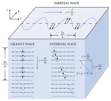
The buoyancy frequency N is proportional to the vertical rate of change in the density of the atmosphere or ocean. It is the natural frequency of oscillation when a volume of dense fluid is displaced into the lighter fluid above or vice versa, and it determines the maximum frequency for internal waves. Those at the buoyancy frequency are called gravity waves and propagate purely in the vertical. Internal waves with intermediate frequencies propagate both horizontally and vertically.

In the midlatitudes, internal waves in the atmosphere and in the ocean are typically high frequency, with periods of 20 hours or less. By contrast, most large‐scale circulation in the ocean and atmosphere varies slowly enough—with periods of months to years—that it may be treated as balanced motion. ¹ In geophysical fluid dynamics terms, balanced motion does not accelerate relative to a fixed point on Earth’s surface. In the atmosphere and ocean, much of the circulation is in thermal‐wind balance, where the pressure resulting from a horizontal density gradient is counteracted by the Coriolis force from Earth’s rotation. Such density gradients, or fronts, in thermal‐wind balance are abundant in the atmosphere and ocean. Atmospheric high- and low-pressure systems—and their ocean equivalent, known as mesoscale eddies—also exist in a state of near thermal‐wind balance. However, if all those systems are balanced, how do they lose energy, decay, and otherwise evolve over time? And how are unbalanced motions such as waves generated?

Internal waves transport significant energy and momentum from their sources, usually near fluid boundaries, into the interior of both the atmosphere and ocean. If the waves have large enough amplitude and small enough scale, they break and dissipate, causing mixing and the acceleration of the balanced flow. A wave’s growth is a consequence of many different mechanisms, including changes to the density structure of the propagating medium, interactions with currents, constructive interference with other waves, and other interactions. In the atmosphere, breaking internal waves contribute to the poleward flow of air in the middle atmosphere (10 km to 80 km high) and therefore help sustain the Brewer–Dobson circulation, wherein air originating at the surface in the tropics cycles to higher altitudes then poleward. Thus, internal waves are a crucial component of weather and climate models. ² Wave breaking is also vitally important in the ocean abyss, below a depth of 2 km, where it drives the mixing of dense water with the lighter waters above (see the article by Adele Morrison, Thomas Frölicher, and Jorge Sarmiento, Physics Today, January 2015, page 27 ). Without that mixing, there would be no overturning of the deep ocean.

Forced generation of internal waves

Have you ever been on a commercial airliner flying over a mountainous region and been warned to return to your seat and buckle up? The sky outside the windows may even have looked clear, but the aircraft soon started shaking and vibrating. That motion was due to a region of clear-air turbulence typically caused by the breaking of a mountain wave. ³ Water or air flow over surface topography, or orography, generates mountain waves, also known as orographic waves; they are the most studied and most prevalent type of internal wave in the atmosphere. Some mountain waves break at low levels near the mountains. Others break in the lower stratosphere, at the typical cruising altitudes of jet airliners, and present a significant aviation hazard.

Mountain-wave generation relies on sufficiently fast near-ground flows and a stably stratified atmosphere, which provides the restoring force on the wave. The topographic obstacle, of length L, pushes the flow, at speed U, up against the force of gravity and over it. If the rate of deflection exceeds the minimum frequency of an internal wave—that is, if U/L > f—then waves are radiated. The nondimensional parameter U/(fL) is known as the Rossby number, Ro, after famed fluid dynamicist Carl-Gustaf Rossby (see the article by Jim Fleming, Physics Today, January 2017, page 50 ), and is one of the most important parameters in meteorology and oceanography.

Mountain waves also occur in the deep ocean, when abyssal currents flow over seafloor topography. However, the currents are slow, with a smaller Rossby number, compared with their atmospheric counterparts. As a result, mountain waves are less common in the ocean than in the atmosphere. Instead, the predominant mechanism for wave generation in the deep ocean is the interaction of the tide with seafloor topography. The gravitational pull of the Moon—and to a lesser extent, the Sun—drives the tide, which is a daily or higher-frequency bulk motion of the water column. That sloshing of stratified water back and forth over the seafloor directly radiates internal waves at the tidal frequency. Tidal generation contributes about 1.5 TW of energy to the ocean wave field; mountain waves ⁴ add only 0.2 TW. A final source of internal waves unique to the ocean has already been mentioned—storms or, more precisely, air currents periodically forcing the ocean surface from above. Storms contribute about 0.3 TW of energy to the ocean’s internal wave field.

The processes described thus far are examples of forced generation of internal waves. They rely on direct high-frequency forcing, such as tides or winds, or interaction with an external body—for example, mountains. Let us turn our attention to the generation of waves without forcing or interaction.

Frontogenesis and spontaneous wave generation

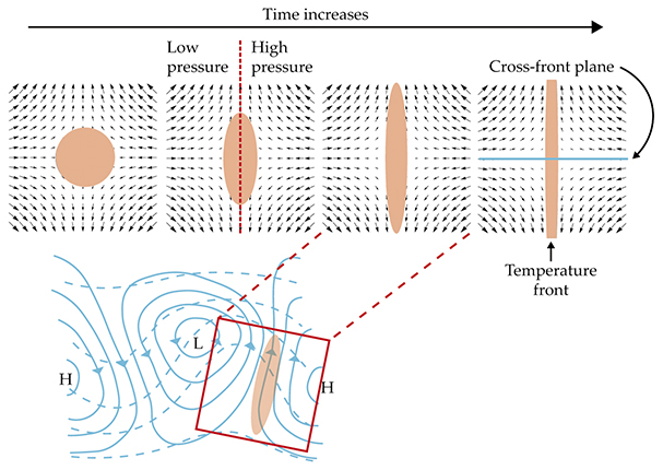
The theory of spontaneous generation originated in the study of weather fronts and their formation, or frontogenesis. Because the fronts are associated with extreme weather such as rain, hail, and snow, frontogenesis has been the focus of much discussion in atmospheric literature over the past century. It occurs in the region between high- and low-pressure systems where the flow is converging, as shown in figure 2. Such flow convergence squeezes and sharpens any existing anomalously steep temperature gradient into an identifiable temperature front.

Figure 2.

In 1968, during his PhD work at the University of Cambridge, Brian Hoskins formulated a mathematical model of frontogenesis. ⁵ It describes how a circulation develops around a front that is initially in thermal-wind balance. The confluence of the high- and low-pressure systems drives circulation with fluid moving up on the warm side and down on the cool side. Figure 3 shows the predicted circulation and temperature structure across the front over time. In the figure, the circulation intensifies as the front sharpens over eight hours. A central tenet of the Hoskins model is that the front remains in a balanced state throughout its evolution. As it sharpens, however, that no-acceleration assumption begins to break down, and internal waves form spontaneously.

Figure 3.

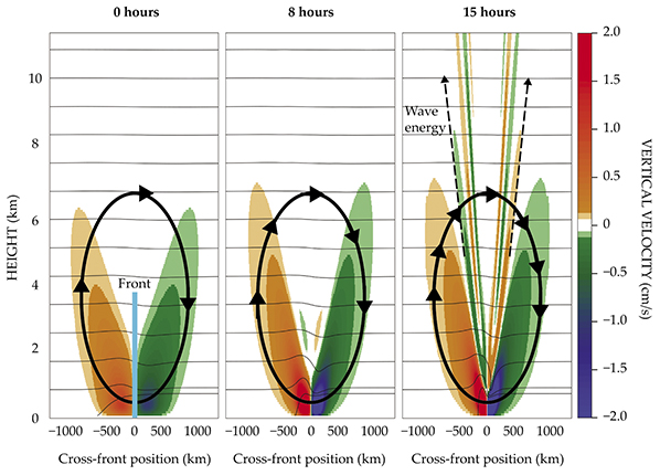
The mathematical description of spontaneous generation requires an extension of the Hoskins model to include the unbalanced cross-frontal acceleration that leads to waves. In a case of academic symmetry, I developed that extended model in 2014 while working on my PhD at the University of Cambridge. ⁶ The extended model departs from the Hoskins model only when the front becomes sufficiently sharp and the convergence of hot and cold regions is sufficiently strong.

Mechanistically, spontaneous internal waves are associated with the rapid vertical displacement of fluid in an otherwise stably stratified environment, similar to mountain waves. Consider a small amount of fluid, a “parcel,” on the warm side of the front. The large-scale convergence pushes the parcel toward the front and then upward, against the restoring force of gravity, into the cooler ambient air above. If that process occurs faster than the minimum frequency of an internal wave, then a wave is generated.

As the front sharpens, the circulation increases, as shown in figure 3. Oncoming convergent flow deflects faster around the front and will reach the minimum-frequency criterion unless frontogenesis is halted by frictional processes or dynamical instabilities. A sharper front leads to a higher amplitude and smaller scale of the generated wave. The convergent flow traps the wave in a location where its horizontal phase speed is equal and opposite to the flow speed, such that the wave appears as a nearly steady feature of the flow. However, the wave propagates vertically and carries energy upward. The idealized mathematical model predicts symmetric wave generation on either side of the front, but in practice, generation occurs preferentially on the warm side, where the surface gradients are larger.

Waves generated spontaneously at atmospheric fronts have a significant effect on the weather. A cold front, shown moving to the right in figure 4, sharpens due to large-scale convergent flow and generates frontal circulation. The rising air ahead of the front forms clouds. When the front sharpens sufficiently, it generates waves (yellow wavy arrows) propagating upward and ahead of the front. Some generated waves, typically smaller-scale ones, propagate directly into the stratosphere. They are responsible for the long, parallel bands of clouds seen on page 34, and they contribute to the large-scale atmospheric circulation when they break and transfer momentum to the balanced flow.

Figure 4.

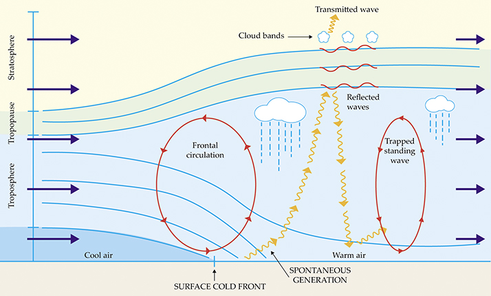
Other generated waves, typically larger-scale ones, contribute to the formation of storms ahead of the advancing cold front. ⁷ The formation relies on a weakly stratified region in the upper troposphere that reflects upward-propagating waves, which then interfere with the reflected waves. A standing wave builds and propagates ahead of the front until it becomes stuck in the oncoming convergent flow. The wave stays ahead of the front and creates one or more narrow bands of vertical motion with typical widths of one to tens of kilometers. Those bands produce clouds, precipitation, and strong winds. ⁸

Frontogenesis and spontaneous generation are not unique to the types of flow described thus far, although those are the most common frontogenetic scenarios. Researchers observe similar effects in fronts with flows whose velocity changes with height. ⁹ All mechanisms of spontaneous generation share a common property: The amplitude A of the generated wave is exponentially small ^{1 , 6} in Rossby number, A ~ e^−1/Ro. Physically, the result means that spontaneous generation exhibits a threshold behavior: Amplitudes are significant only once the Rossby number exceeds a critical value, which theory estimates to be 0.15–0.20. An immediate consequence is that spontaneous generation is localized in time and space to regions that satisfy the threshold.

The ocean: Spontaneous or stimulated?

One flow regime in which the Rossby number threshold is routinely exceeded is the ocean submesoscale, a scatter of density fronts and eddies with lateral scale of less than 10 km and localized primarily in the upper 50 m of the ocean. ¹⁰ Large strains and shears from the surrounding turbulent flow prime the density fronts at the submesoscale for spontaneous generation. Recent numerical models attempted to quantify the global energy transfer to waves associated with spontaneous generation in that region. ^{11 , 12} Those studies found that although local energy flux from spontaneously generated waves may be large, the area-averaged values are relatively small and account for 0.03 TW of wave generation globally, or 1/10 of the 0.3 TW due to winds. Spontaneous generation contributes to, but is not a dominant source of, wave energy in the ocean.

Spontaneous generation is one mechanism for transferring energy from balanced flow to unbalanced waves. The search for other links between balanced and unbalanced flow is a major focus of the oceanography community. Recent work proposes a new mechanism called stimulated emission, the transfer of energy from balanced flow to a preexisting wave rather than the generation of new waves. Stimulated emission does not require a large Rossby number and therefore transfers much more energy. Theorists have developed models to describe the dynamics of stimulated emission at low Rossby number, where the balanced flow is well understood. 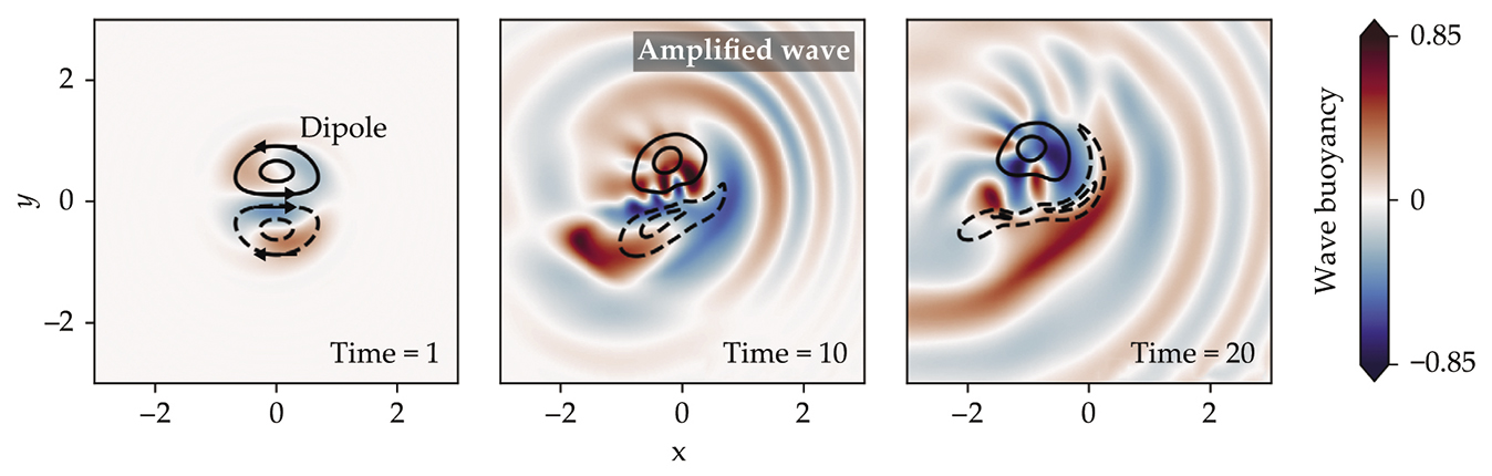^{13 , 14} The results of one model are shown in figure 5. The model starts with a uniform wave and a localized dipole, or double eddy. The dipole locally squeezes and amplifies the gradients of the wave, and the wave’s energy increases with time as the dipole loses energy. Studies using more realistic models ^{15 , 16} suggest that stimulated emission occurs frequently in the ocean, especially in response to wind forcing. One study ¹⁵ reported a 30% enhancement, or about 0.1 TW globally, in the energy in wind-generated internal waves, at the expense of balanced flow.

Figure 5.

Outlook

Many questions remain about the importance and role of spontaneous generation and related processes, such as stimulated emission, in creating internal waves. Those questions have important consequences for the fields of oceanography, meteorology, and climate science.

In the ocean context, recent work on spontaneous and stimulated emission showed that internal waves sometimes gain energy from and lose energy to balanced flows. ¹² That body of work shifts the field away from the classical paradigm that winds, tides, and topography force internal waves, which then directly dissipate their energy and drive mixing. The energy pathways between generation and dissipation are considerably more complex, and understanding them will lead to better constraints on the variability and location of wave-driven mixing and the associated effects on ocean circulation.

In the atmosphere context, researchers are interested in quantifying nonorographic sources of internal waves. Midlatitude fronts are major sources of nonorographic waves, and spontaneous generation is one mechanism for generating those waves. Although nonorographic waves are locally less intense than mountain waves, which are highly localized with large amplitudes, their cumulative contribution may be comparable. ¹⁷ They are often not included in global atmospheric models because of the uncertainty in their spatial and temporal distribution. Theoretical advances are starting to correct the situation, but more work is needed to translate idealized theoretical models into more realistic settings. Given that nonorographic waves may contribute substantially to circulation in the middle atmosphere, their inclusion in models should improve seasonal and multiyear forecasting.

Researchers have made significant progress in their understanding of internal waves in the ocean and atmosphere through a combination of observational, modeling, and theoretical advances, only a small subset of which are discussed here. Spontaneous generation is one element of that work, which broadly examines the interactions of unbalanced flows with the large-scale balanced flows that dominate our climate and weather.

References

1. J. Vanneste, Annu. Rev. Fluid Mech. 45, 147 (2013). https://doi.org/10.1146/annurev-fluid-011212-140730
2. D. C. Fritts, M. J. Alexander, Rev. Geophys. 41, 1003 (2003). https://doi.org/10.1029/2001RG000106
3. A. D. Elvidge et al., Meteorol. Appl. 24, 540 (2017). https://doi.org/10.1002/met.1656
4. A. F. Waterhouse et al., J. Phys. Oceanogr. 44, 1854 (2014). https://doi.org/10.1175/JPO-D-13-0104.1
5. B. J. Hoskins, F. P. Bretherton, J. Atmos. Sci. 29, 11 (1972). https://doi.org/10.1175/1520-0469(1972)029<0011:AFMMFA>2.0.CO;2
6. C. J. Shakespeare, J. R. Taylor, J. Fluid Mech. 757, 817 (2014). https://doi.org/10.1017/jfm.2014.514
7. D. M. Schultz, Mon. Weather Rev. 133, 2449 (2005). https://doi.org/10.1175/MWR2987.1
8. C. J. Shakespeare, J. Atmos. Sci. 73, 2837 (2016). https://doi.org/10.1175/JAS-D-14-0294.1
9. F. Lott, R. Plougonven, J. Vanneste, J. Atmos. Sci. 69, 2134 (2012). https://doi.org/10.1175/JAS-D-11-0296.1
10. J. C. McWilliams, Proc. R. Soc. A 472, 20160117 (2016). https://doi.org/10.1098/rspa.2016.0117
11. T. Nagai et al., J. Phys. Oceanogr. 45, 2381 (2015). https://doi.org/10.1175/JPO-D-14-0086.1
12. C. J. Shakespeare, A. M. Hogg, J. Phys. Oceanogr. 48, 343 (2018). https://doi.org/10.1175/JPO-D-17-0153.1
13. C. B. Rocha, G. L. Wagner, W. R. Young, J. Fluid Mech. 847, 417 (2018). https://doi.org/10.1017/jfm.2018.308
14. J.-H. Xie, J. Vanneste, J. Fluid Mech. 774, 143 (2015). https://doi.org/10.1017/jfm.2015.251
15. R. Barkan, K. B. Winters, J. C. McWilliams, J. Phys. Oceanogr. 47, 181 (2017). https://doi.org/10.1175/JPO-D-16-0117.1
16. S. Taylor, D. Straub, J. Phys. Oceanogr. 46, 79 (2016). https://doi.org/10.1175/JPO-D-15-0060.1
17. R. Plougonven, F. Zhang, Rev. Geophys. 52, 33 (2014). https://doi.org/10.1002/2012RG000419
More about the authors
Callum Shakespeare is a research fellow at the Australian National University in Canberra.