Locating lightning
DOI: 10.1063/PT.3.3869

Most of us have experienced air travel delays or other aggravation provoked by lightning and thunderstorms. Yet the headache of extra time on the ground pales in comparison to the threat to ground staff at airports. Moreover, low-level wind shear caused by thunderstorms is a well-documented killer, having caused the tragic crash of Delta Air Lines Flight 191 on its final approach to the Dallas/Fort Worth International Airport in August 1985. Modern lightning location systems (LLSs) now enable more precise warnings to airport personnel, as I personally experienced during a 45-minute flight delay at an airport whose lightning warning system I helped to configure.
The evolution of modern LLSs dates back approximately 40 years, when early systems aided the deployment of firefighting aircraft and crews to combat wildfires over wide areas of western North America. 1 Nowadays, in addition to locating the origins of lightning-caused wildfires and helping to protect airport personnel, LLSs locate faults on electric power grids and validate claims of lightning damage in the insurance industry. A few months ago, LLSs helped establish that lightning strikes are unusually high above two busy shipping lanes; presumably the increased activity is caused by ships’ aerosol emissions. (See Physics Today, November 2017, page 20 .) LLSs operate worldwide at regional to global scales. 2 , 3 In many cases they can locate lightning to within 100 meters.
Even in the early days, electric utilities rapidly adopted LLS data to reduce the frequency and duration of outages and to make improvements to transmission-line segments found to be particularly susceptible to lightning-caused problems. 4 Power outages are almost always frustrating and inconvenient, but sometimes they are much more than that. The infamous 1977 blackout in New York City ultimately affected approximately 9 million people and resulted in economic damage in excess of $300 million. 5 It was initiated by a lightning strike. In the decades since, however, the likelihood of such lightning-induced catastrophes has been dramatically reduced through the use of LLSs.
In this article I describe the general types of LLSs, the data they provide, and how those data are used. Broadly speaking, LLSs fall into one of two categories: networks of ground-based sensors that are sensitive to RF emissions or satellite-based sensors that observe so-called optical emissions, though they’re really in the near-IR. The different types of LLSs provide complementary information about lightning flashes and their parent thunderstorms. Box
Spotting cloud-to-ground strokes
To locate transmission-line faults or to validate claims of lightning damage, an LLS has to determine with high confidence which specific discharge processes are cloud-to-ground (CG) strokes and to register with high precision where they occur. Figure
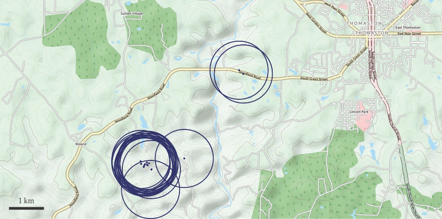
Figure 1.

Fifteen strokes. In April 2015, during a cloud-to-ground flash outside Thomaston, Georgia, 15 strokes contacted ground, but not all at the same location. The small dots represent the best estimates of position provided by a ground-based lightning location system, and the nearly circular shapes surrounding them depict the position uncertainty at the 99% confidence level. Two strokes occurred about 3 km northeast of their nearest neighbor, well beyond its 99% confidence limit. Two other strokes occurred roughly 1 km from the main cluster, but they were not statistically distinguishable from the main cluster with 99% confidence.
Precise determinations of where CG strokes contact ground can be obtained only from ground-based LLSs that sense RF emissions primarily at frequencies below 500 kHz. Such systems are generically called low-frequency (LF) LLSs (reference spells out more precise terminology). To determine the location of individual emissions, all modern LF LLSs use the arrival times of the detected signals at multiple sensors, and many use the arrival directions as well. Lightning sensors that operate primarily in the 1–500 kHz range register waves whose wavefronts propagate along the ground, bending continuously in response to induced ground current. Such sensors can detect lightning hundreds of kilometers away, and thus, the sensors themselves may be separated by several hundred kilometers. Waves with frequencies below about 50 kHz can also propagate in the waveguide formed by the ionosphere and the ground. The confining effect of the waveguide enables sensors to detect those very low frequency (VLF) waves at distances of thousands of kilometers; VLF sensors can thus be more widely spaced than detectors that are also sensitive to higher frequencies.
Box 1. Coming to terms with lightning
A lightning flash typically lasts no longer than a second. It consists of various discharge subprocesses, most of which occur in the thunderstorm cloud. In fact, about 75% of all lightning flashes occur entirely within a cloud or between clouds. Those are called cloud flashes or IC (intracloud or intercloud) flashes. The remaining 25% include one or more cloud-to-ground (CG) return strokes (often called CG strokes)—high-current impulses that make contact with the ground. Any flash that contains at least one CG stroke is, by definition, a CG flash. For a specified time interval, the set of all IC and CG flashes taken together is usually called total lightning. For additional details of lightning discharge processes and terminology, see reference .
Lightning location systems (LLSs) are designed to provide the times and locations of lightning flashes or flash subprocesses. Typically, their performance is evaluated in terms of two fundamental characteristics: the detection efficiency and location accuracy. Detection efficiency can refer to either the fraction of flashes detected by the LLS or a particular class of subprocess such as CG strokes. Location accuracy quantifies how well an LLS determines position. It is typically given as a single value, such as the median of the distribution of position uncertainties. Depending on their specific characteristics, ground-based LLSs may also be able to differentiate between CG strokes and IC processes, estimate the peak currents carried by CG strokes, or determine the polarity of the discharge—that is, whether the current flows upward or downward. Very dense LLSs may furnish an estimate of the altitude of RF emission sources in addition to determining the source’s latitude and longitude. In those cases of enhanced capabilities, the standard measures of detection efficiency and location accuracy are joined by such additional measures of performance as the accuracy of CG versus IC differentiation or altitude determination.
To some extent, ground-based LF LLSs are total lightning LLSs, capable of observing both CG and intracloud or intercloud (together called IC) events. Of the two, the CG strokes are the stronger emitters of LF radiation. The IC processes that are most effectively detected by LF LLSs are vertically oriented and carry currents of at least 1 kA. Typical detection efficiencies of LF LLSs that rely mainly on ground waves are 70–90% for CG strokes, 90–100% for CG flashes, and 50% or more for IC flashes. The median location accuracy of CG strokes can be as good as 100–200 m in ground-wave-detecting LLSs and 2–10 km for LLSs that rely on VLF waveguide propagation.
Systems that operate in both the LF and VLF can estimate the peak current of a CG stroke and determine whether positive or negative charge touches ground. Peak current can typically be obtained with an accuracy of 15–30%, depending on the frequency range that can be sensed by the LLS. Those LLSs can also differentiate between CG strokes and IC processes either by means of the characteristics of the received waveform shapes or by an estimate of the altitudes of the emission sources. The differentiation accuracy depends on the differentiation technique, the sensor spacing, and the frequency range observed. In the best cases, it can exceed 90%.
Storm clues
The long-distance propagation of VLF signals enables lightning location in remote areas where there exists little or no other meteorological information such as radar scans, surface observations, or upper-atmospheric data typically obtained with radiosondes flown on weather balloons. One example concerns Typhoon Haiyan. In November 2013, Haiyan developed rapidly off the east coast of the Philippines; ultimately it would become the strongest tropical cyclone known to make landfall up to that time. Figure
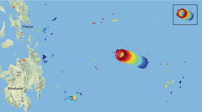
Figure 2.

Lightning during the rapid development of Typhoon Haiyan on 7 November 2013. Color indicates time, from blue (8:00am local time) to red (1:00pm). The concentrated area of lightning on the right, the eyewall, propagates west–northwest during the five-hour observation period. The inset at the upper right shows a two-hour segment, zoomed in on the eyewall, that better reveals the cylindrical form of the eyewall and the calm eye at the center of the storm.
Lightning reveals the existence of updrafts powerful enough to support the dominant mechanism of charge separation in thunderstorms. The process, further described in box
Lightning is an observable manifestation of those energetic kinetic and thermodynamic phenomena. The relationship between electrified storms in the eyewall and the development of exceptionally vigorous tropical cyclones such as Haiyan remains incompletely understood. 6 With the aid of long-distance LLS observations, it is becoming clearer that the production of lightning and the various stages of tropical cyclone development are related in complex ways and that those relations kick in as early as the tropical depression stage. 7
In nontropical thunderstorms, a rapid increase in the rate of total lightning is thought to be a harbinger of severe weather. More and more, LLSs are being used to detect those increases in the hope of improving the lead times of severe weather warnings. 8
Lightning mapping
The lightning-producing area of thunderstorm clouds can be tens or even hundreds of kilometers across. Aircraft and spacecraft operators need information about the full extent of that area, in part because of the dangers associated with the turbulence and icing produced by thunderstorms. Another significant worry is the possibility that a craft might set off lightning when passing through an electrified cloud. The threat of triggering lightning in clouds that otherwise would not generate flashes was first discovered with the 1969 Apollo 12 lightning incident at the John F. Kennedy Space Center. 9 The instrumentation used to detect electrified clouds that do not produce lightning is described in reference .
Lightning location systems that operate at low frequency cannot observe the rich channel structure of a lightning flash. LLSs that do have that capability, called lightning mapping systems, are usually space-based optical sensors or ground-based networks of sensors sensitive to RF emissions in the high-frequency (HF; 3–30 MHz) to very high frequency (VHF; 30–300 MHz) bands. For example, the US Air Force’s 45th Weather Squadron, which provides forecasts over the Kennedy Space Center, uses ground-based lightning mapping systems as part of its comprehensive lightning warning process. As described in greater detail below, ground-based VHF systems provide spatial detail. But they typically cover only about the same area as a weather radar. Space-based sensors can cover vastly greater territory but with lower resolution.
For the most part, VHF emissions from lightning flashes fall into one of two categories: microsecond-scale impulsive events or quasi-continuous bursts with durations of tens to hundreds of microseconds.
11
The impulses are most easily located via time-of-arrival measurements, whereas the bursts are better suited to direction-of-arrival measurements obtained by means of VHF interferometry. The number of VHF emission sources observed in a lightning flash can range from tens to more than 10 000. Admittedly, not all subflash processes generate readily detectable VHF emissions,
12
and the specific subflash processes responsible for each type of VHF emission are different. Nonetheless, the majority of 100-m-scale channel structures in lightning flashes can be located using impulsive or quasi-continuous VHF emissions, and the flash detection efficiency of VHF LLSs is virtually 100% for both IC and CG flashes. Figure
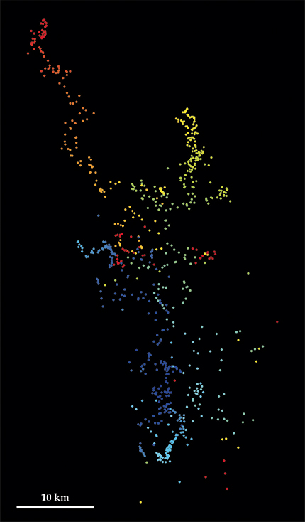
Figure 3.

Lightning mapping. A ground-based lightning location system observing in the very high frequency band determined the horizontal positions of several hundred emissions in this single flash, which occurred in the south-central US. Color, from dark blue (earliest) to red, indicates time within the flash.
Due to the sharpness and submicrosecond duration of impulsive VHF emissions, time-of-arrival LLSs can locate them in all three dimensions with an accuracy of tens of meters. The location accuracy of the quasi-continuous emissions determined by VHF interferometry is a few kilometers. One reason for the reduced accuracy is the necessity of integrating over the time of the emission. Others are the wide intersensor separation and the nature of the angle measurements associated with VHF interferometry.
In contrast to ground-wave signals at frequencies below 500 kHz, VHF emissions do not enable the assessment of the peak current of a CG stroke or the polarity of IC and CG lightning—that is, whether the current flows upward or downward. Nor do VHF systems readily enable differentiation between CG strokes and IC processes. Time-of-arrival VHF LLSs do resolve altitude. In practice, however, such resolution does not differentiate between CG strokes and IC processes because, close to the ground, the probability of signal blockage by terrain features or buildings increases. For that reason, researchers frequently combine data from VHF LLSs with observations from lower-frequency LLSs to provide robust CG stroke identification.
Signal blockage is the most significant limitation of VHF LLSs; the VHF signals are largely limited to line-of-sight propagation. Thus ground-based VHF LLSs are restricted in coverage to an area within a few hundred kilometers of the center of the system, and sensor spacing is limited to at most about 100 km for VHF interferometry or tens of kilometers for time-of-arrival measurements.
Satellite systems
The best way to obtain spatial mapping of lightning over very large areas is via satellite. Mapping observations with satellite-borne optical lightning sensing started more than 20 years ago, when NASA’s Optical Transient Detector aboard the OrbView-1 satellite began collecting data. 13 In November 2016 the US launched the Geostationary Lightning Mapper (GLM) on GOES-16, the first geostationary satellite to contain an optical lightning sensor. 14 A few weeks later, China launched its Fengyun-4-01 satellite, which also carries an optical lightning sensor. 15
Those and other space-based sensors operate by detecting atomic spectral-line emissions; the light is scattered out of thunderclouds after being generated by current-bearing channels in lightning flashes whose temperatures reach thousands of kelvin. The GLM and its predecessor low-Earth orbiting instruments measure the 777.4-nm-wavelength light emitted by singly ionized atomic oxygen.
For a space-borne sensor, the detection efficiency is defined as the percentage of total lightning flashes that the sensor observes. It depends on the time of day, because the sensors have to subtract backscattered sunlight from the cloud tops to detect lightning signals during the day. The detection efficiency of the Lightning Imaging Sensor (LIS), one of GLM’s predecessors, was roughly 70% at midday and 90% at night. 13 The location accuracy of space-based sensors is dictated largely by the pixel size projected onto the ground and the accuracy with which the satellite image can be converted to a ground location. For the GLM, the pixel resolution is 8 km at the equator and 14 km near the edge of the field of view at ±52° latitude.
Because the light observed by the LIS and other similar devices is scattered many times in clouds, satellite-borne sensors do not differentiate between CG strokes and IC processes, nor do they provide estimates of peak current, polarity, or altitude. They do, however, observe the intensity of optical emission, which is not observable by ground-based LLSs. The fuller representation of lightning characteristics given by a combination of satellite- and ground-based observations can have important practical implications.
Figure
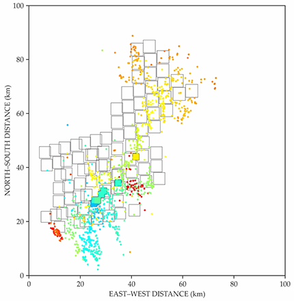
Figure 4.

One cloud flash over the south-central US, as seen by three lightning location systems (LLSs). The open gray squares represent observations made by the satellite-borne Lightning Imaging Sensor. The small dots show sources of very high frequency emission, and the colored, filled-in squares show cloud discharges spotted by an LLS operating at very low frequency and low frequency. Color coding indicates time from the beginning (blue) of the 1.4-second flash.
For the particular flash of figure

Lightning over Tucson, Arizona. (Copyright Warren Faidley/123RF.com.)
The figure neatly encapsulates differences between observations from different types of LLSs, and it is also suggestive of the differing needs of LLS users. Only LLSs operating in the LF and VLF bands can locate CG strokes precisely and distinguish them from IC events, a combination of features that is crucial for those working in the energy and insurance sectors. In addition, LF systems have the advantage of covering large territories. VHF mapping systems provide data from the entire extent of a flash with excellent resolution, information that is valuable for operations carried out, for example, at the Kennedy Space Center. Satellite-borne sensors provide much greater coverage. Their ability to map lightning over remote areas can be valuable to meteorologists who otherwise would have little or no data.
Remote areas are not of interest just to meteorologists. Wildfires frequently start in remote areas. But wildfires are initiated by CG strokes, and space-borne optical sensors cannot differentiate between CG and IC flashes. It is a combination of satellite data and observations from LF systems that often best serves the needs of LLS users, in particular those who require detailed information about CG strokes for their analyses of forest-fire ignition, airport safety, or damage to electrical systems.
Box 2. Electrification of thunderclouds
Before lightning can flash, charge must separate in a cloud. Although researchers have proposed many mechanisms for that large-scale charge separation, 17 field observations of electric-field changes due to lightning, balloon-borne soundings of the charge structure of thunderstorms, laboratory experiments, and numerical models have gradually led to a consensus: The dominant charge-separation mechanism takes place in the presence of supercooled liquid-water droplets and involves collisions between small ice crystals and soft, snow pellets called graupel. The essence of the process, called the relative growth rate mechanism, is that a small amount of positive charge is carried away by whichever of the two colliding particles is growing faster.
Why is the generation of charge related to growth rate? The key is that ice particles grow in large part by vapor deposition, a process that is disorderly in thunderstorm clouds due to the presence of supercooled liquid droplets that maintain a water-vapor concentration that is slightly supersaturated with respect to ice. As an ice particle grows in such an environment, it incorporates ionic defects arising from the dissociation of water into H+ and OH− ions. Bond rotations and proton transfers enable the H+ ions to move within the ice-crystal lattice, but the OH− defects are essentially immobilized by hydrogen bonds to surrounding molecules.

The ionic-defect concentration is related to the growth rate, so whichever particle is growing faster by vapor deposition has a higher concentration of defects. Because the OH− ions are stuck where they form, whereas the H+ are mobile, an overall difference in defect concentration translates to a difference in near-surface negative-charge density. Collisions between small ice crystals and graupel pellets last just long enough and generate just enough near-surface melting that a small amount of liquid is exchanged during the collisions. Overall, the associated mixing transfers a small amount of OH− from whichever particle has the larger concentration—the one that had been growing more rapidly—to the one with the smaller concentration.
As mentioned earlier, supercooled liquid maintains a water-vapor concentration that is supersaturated with respect to ice. The reason is simply that in typical thunderstorm conditions, the vapor pressure over liquid water is higher than that over ice. The supercooled droplets also accumulate on the ice crystals and especially the graupel pellets.
The figure shows the results of a highly simplified relative growth rate model, in which a single ice crystal interacts with a single graupel pellet. The blue area shows the range of temperature and liquid-water content for which the ice crystal is the faster-growing particle and thus would transfer some of its OH− to a graupel pellet in a collision. In the small red area corresponding to relatively high temperatures and liquid-water content, the graupel grows faster. The vertical axis gives the base-10 logarithm of the ratio of the graupel-to-crystal defect accumulation rate.
I thank Daile Zhang of the University of Arizona for assistance with obtaining and decoding data from the flash shown in figure
References
1. E. P. Krider et al., Bull. Am. Meteorol. Soc. 61, 980 (1980). https://doi.org/10.1175/1520-0477(1980)061<0980:LDFSFF>2.0.CO;2
2. A. Nag et al., Earth Space Sci. 2, 65 (2015). https://doi.org/10.1002/2014EA000051
3. R. Said, Weather 72, 36 (2017). https://doi.org/10.1002/wea.2952
4. K. L. Cummins, W. A. Chisholm, Transm. Distrib. World 67(11), 52 (2015).
5. J. L. Corwin, W. T. Miles, Impact Assessment of the 1977 New York City Blackout, DOE EC-77-C-01-5013, Systems Control Inc (July 1978).
6. A. O. Fierro, in Advanced Numerical Modeling and Data Assimilation Techniques for Tropical Cyclone Prediction, U. C. Mohanty, S. G. Gopalakrishnan, eds., Springer (2016), p. 197.
7. M. DeMaria et al., Mon. Weather Rev. 140, 1828 (2012). https://doi.org/10.1175/MWR-D-11-00236.1
8. C. J. Schultz et al., Weather Forecast. 32, 275 (2017). https://doi.org/10.1175/WAF-D-15-0175.1
9. R. Godfrey et al., Analysis of Apollo 12 Lightning Incident, NASA (February 1970).
10. J. Montanya, J. Bergas, B. Hermoso, J. Electrost. 60, 241 (2004), and references therein. https://doi.org/10.1016/j.elstat.2004.01.009
11. K. L. Cummins, M. J. Murphy, IEEE Trans. Electromagn. Compat. 51, 499 (2009). https://doi.org/10.1109/TEMC.2009.2023450
12. E. R. Williams, Plasma Sources Sci. Technol. 15, S91 (2006). https://doi.org/10.1088/0963-0252/15/2/S12
13. D. J. Cecil, D. E. Buechler, R. J. Blakeslee, Atmos. Res. 135–136, 404 (2014). https://doi.org/10.1016/j.atmosres.2012.06.028
14. S. J. Goodman et al., Atmos. Res. 125–126, 34 (2013). https://doi.org/10.1016/j.atmosres.2013.01.006
15. J. Yang et al., Bull. Am. Meteorol. Soc. 98, 1637 (2017). https://doi.org/10.1175/BAMS-D-16-0065.1
16. V. A. Rakov, Fundamentals of Lightning, Cambridge U. Press (2016).
17. C. Saunders, Space Sci. Rev. 137, 335 (2008). https://doi.org/10.1007/s11214-008-9345-0
More about the authors
Martin Murphy is a senior scientist at Vaisala Inc in Louisville, Colorado.


