Improving students’ understanding of quantum mechanics

Richard Feynman once famously stated that nobody understands quantum mechanics. He was, of course, referring to the many strange, unintuitive foundational aspects of quantum theory such as its inherent indeterminism and state reduction during measurement according to the Copenhagen interpretation. But despite its underlying fundamental mysteries, the theory has remained a cornerstone of modern physics. Most physicists, as students, are introduced to quantum mechanics in a modern-physics course, take quantum mechanics as advanced undergraduates, and then take it again in their first year of graduate school. One might think that after all this instruction, students would have become certified quantum mechanics, able to solve the Schrödinger equation, manipulate Dirac bras and kets, calculate expectation values, and, most importantly, interpret their results in terms of real or thought experiments. That sort of functional understanding of quantum mechanics is quite distinct from the foundational issues alluded to by Feynman.

Extensive testing and interviews demonstrate that a significant fraction of advanced undergraduate and beginning graduate students, even after one or two full years of instruction in quantum mechanics, still are not proficient at those functional skills. They often possess deep-rooted misconceptions about such features as the meaning and significance of stationary states, the meaning of an expectation value, properties of wavefunctions, and quantum dynamics. Even students who excel at solving technically difficult questions are often unable to answer qualitative versions of the same questions.

A growing number of physics education researchers, borrowing heavily from tools and methods developed for introductory-level physics, have begun to investigate and address issues related to students’ understanding of quantum mechanics. ^1–3 One interesting result is that most of the students’ difficulties are universal. ^3,4 That is, they are independent of teaching styles, textbooks, institutions, and students’ backgrounds. And patterns of incorrect notions of quantum mechanics are analogous to those that have been well-documented for introductory physics courses.

In this article we underscore the need for physics education research in quantum mechanics by illustrating some of the most pervasive difficulties students have. We then survey tools that are being developed to help improve and deepen students’ understanding of this important subject.

Students’ misconceptions

Several studies have investigated misconceptions of students who were exposed to quantum mechanics in modern-physics courses. The difficulties illustrated in the following examples were identified with the help of research-validated surveys administered to 89 advanced undergraduates and more than 200 first-year physics graduate students from seven universities. ³ Topics covered included general properties of the wavefunction, time dependence of the wavefunction, probabilities for measurement outcomes, and expectation values and dynamics for energy and other observables. Numerous in-depth interviews followed the administration of the survey.

In one survey question, students were asked to write down the most fundamental equation in quantum mechanics. Only 32% of students indicated the time-dependent Schrödinger equation, HΨ — iħ ∂Ψ/∂t, or equivalent statements involving commutation relations. In contrast, 48% of students wrote down the time-independent Schrödinger equation, HΨ = EΨ. We note that Erwin Schrödinger received his Nobel Prize for the fundamental, time-dependent equation. As evidenced by the following two questions, the students’ sense that the time-independent equation is fundamental is closely linked to a number of their difficulties and misconceptions about quantum mechanics.

One of the survey questions asked students to

Consider the following statement: “By definition, the Hamiltonian acting on any allowed state of the system Ψ will give the same state back, i.e., HΨ = EΨ, where E is the energy of the system.” Explain why you agree or disagree with this statement.

Figure 1 summarizes the responses that students gave. The correct answer was given by 29% of students: The statement is true only if Ψ is a stationary state. Among the incorrect answers, a full 39% of students wrote that the statement is true unconditionally. Typically, those students were supremely confident of their answers. For example, one wrote: “Agree. This is what 80 years of experiment has proven. If future experiments prove this statement wrong, then I’ll update my opinion on this subject.”

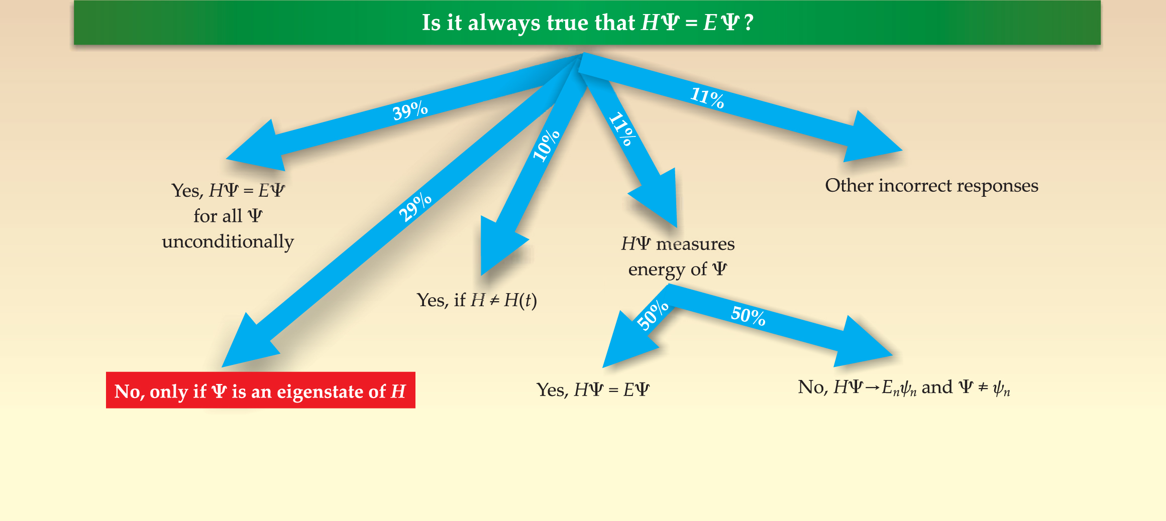
A total of 11% of the students believed that any statement involving a Hamiltonian H acting on a state Ψ describes a measurement of the state’s energy. Armed with that philosophy, some agreed with the statement they were asked to consider. Others disagreed, stating that the wavefunction collapsed after the measurement so that HΨ = E_nψ_n , where ψ_n is the stationary state into which the wavefunction collapsed.

Another 10% of students claimed that the statement is true only if H is not explicitly time dependent. In that case, they argued, the energy of the system is conserved and hence HΨ = EΨ. The argument is incorrect since Ψ need not be an eigenstate of H, even if H is time independent.

A second question illustrates students’ misconceptions about expectation values and quantum dynamics for an electron in an infinite square-well potential.

The wavefunction of an electron in a one-dimensional infinite square well of width a, x∈ (0, a), at time t = 0 is given by $\mathrm{\Psi }(x,0)=\sqrt{2/7}{\psi }_1\left(x\right)+\sqrt{5/7}{\psi }_2\left(x\right)$, where ψ ₁(x) and ψ ₂(x) are the ground state and first excited stationary state of the system. ${\psi }_n\left(x\right)=\sqrt{2/a}\sin (n\pi x/a)$, E_n = n ² π ² ħ ²/(2ma ²), where n = 1, 2, 3, ….) [The original question included a potential energy diagram and slightly different notation.]

Only 43% of the students correctly responded to part a of the question. The most common mistake, made by 31% of the students, was to write a common phase factor for both terms along the lines of Ψ(x, t) = Ψ(x, 0)e ^−iEt/ħ .

Follow-up interviews confirmed that students had trouble distinguishing the properties of stationary and nonstationary states. Several students thought that the time dependence always took the form of a decaying exponential. During interviews, some of them explained their choice by insisting that the wavefunction must decay with time because “that is what happens for all physical systems.” Interestingly, 9% of the students wrote that Ψ(x, t) should not have any time dependence whatsoever; during interviews, some tried to justify their claim by pointing out that the Hamiltonian is time independent.

Part b of the question got more correct responses, 67%, than any other segment of the survey; that success makes a comparison with the responses for part c particularly revealing. It shows that students could calculate probabilities for the outcome of measurements, but many were unable to use that information to determine an expectation value.

Many students who answered part b correctly, including those who also answered c correctly, calculated the expectation value of the energy 〈E〉 by brute-force methods: They first wrote $〈E〉={\int }_{-\infty }^{+\infty }\Psi *H\Psi dx$ , then expressed Ψ(x, t) in terms of the two energy eigenstates, then acted on the eigenstates with the Hamiltonian, and finally used orthogonality to obtain their answer. Some of those who missed part b got lost early in the process. Others did not remember such mechanical steps as taking the complex conjugate of the wavefunction, exploiting the orthogonality of stationary states, or using the proper integration limits.

Interviews revealed that many students did not know or recall the interpretation of the expectation value as an ensemble average, and did not realize that the expectation value asked for in part c could be calculated more simply by taking advantage of their part-b answer. Some, including students who correctly evaluated Ψ(x, t) in part a, believed that the expectation value of energy should depend on time. Other questions posed to students confirmed that many of the difficulties they have are both conceptual and deep rooted.

Instructors are often surprised at how students who do well on quantitative problems have difficulty when essentially the same problems are posed qualitatively. Often, qualitative understanding of quantum mechanics is much more challenging than facility with the technical aspects. Similar to “plug and chug” problems in introductory physics, strict quantitative exercises in quantum mechanics often fail to provide adequate opportunity for reflection on the problem-solving process and for drawing meaningful inferences. Based on our ongoing research, we believe that learning tools that combine quantitative and qualitative problem solving can be effective in helping students learn quantum mechanics.

Inappropriate generalization

The universal nature of students’ misconceptions about quantum mechanics is somewhat surprising, given the abstract nature of the subject. Misconceptions in introductory-level physics are often viewed as originating from incorrect worldviews. But it is hard to explain conceptual difficulties in quantum mechanics in that fashion.

Shared misconceptions in quantum mechanics can be traced in large part to incorrect generalizations of concepts learned earlier, either in classical mechanics or in quantum mechanics. For example, many students believe that an object with a label x is orthogonal to or cannot influence an object with a label y. According to this belief, eigenstates of the spin operators S_x and S_y are orthogonal. The improper generalization originates from properties of classical vectors.

Here’s another example: Many students believe that if the expectation value of a physical observable is zero in the initial state, its expectation value cannot have any time dependence. That misconception is related to a similar one in introductory physics: If the velocity of an object is zero, its acceleration must be zero as well.

Sometimes students fail to distinguish between closely related concepts and make inappropriate generalizations in a purely quantum context. We have already noted that many students claim that the time-independent Schrödinger equation is always true. Other examples of inappropriate generalizations are more subtle.

Many students, for instance, believe that the expectation value of any time-independent Hermitian operator is also time-independent if the initial state is an eigenstate of that operator. This belief can be regarded as an incorrect generalization from two true statements; namely, the expectation value of a time-independent Hermitian operator in a stationary state doesn’t change with time, nor does the expectation value of a Hermitian operator, in any state, that commutes with the Hamiltonian.

A related false belief is that measurement of any physical observable causes the system to get “stuck” in the measured eigenstate forever unless an external perturbation is applied. Again, the statement is true only for observables whose operators commute with the Hamiltonian, but students seem to generalize that property of measurement to include all observables.

How can instruction in quantum mechanics be modified to reduce the difficulties that students have? One option is that instructors can take advantage of computer-based learning tools. (The box on page 44 describes ComPADRE, a digital library designed to help instructors find the resources they need.) But teaching with technology, without a sound pedagogy, does not automatically yield significant educational gains (see the article by Carl Wieman and Katherine Perkins, Physics Today, November 2005, page 36 ). An important first step in developing strategies that can help students is to be aware of the difficulties they typically face while learning quantum mechanics. Later in this article, we discuss how tutorials embedded in a coherent curriculum are well suited to direct targeting of the misconceptions that have been identified through research. But first we turn to simulations available for quantum mechanics classes and say a few words about recently developed laboratory experiments.

Experiments, virtual and real

Fast and realistic computer-based visualization tools can play a key role in various advanced-level topics, including quantum mechanics. The computational power of desktop and laptop computers is more than sufficient to run such simulations, and many heretofore inaccessible topics in quantum mechanics can now be discussed and exemplified in concrete terms. Most simulations can be run either as standalone applications or within Web browsers and are written using metalanguages and virtual machines that ensure that the software is platform independent and adaptable.

One of the first quantum simulations for instructional purposes was created in 1967 by Abraham Goldberg and colleagues, who simulated scattering of Gaussian wavepackets off different wells and barriers. ⁵ Computer-generated probability densities were displayed on a cathode-ray tube and photographed, then the successive frames were turned into a movie. Numerous textbooks, even to this day, have referenced or reprinted those images, and other texts have extended the work by including more scenarios and depicting time development with successive images, ⁶ QuickTime movies, ⁷ or even interactive simulations. ⁸

The Open Source Physics (OSP) project, with support from NSF, has developed a freely available, open-source Java library, along with documentation, that helps instructors to develop physics software and distribute Web-based curricular material. ⁹ The OSP technology was originally designed for the teaching of computational physics, but it has been used to write and organize curricular material for classical mechanics, electromagnetism, statistical physics, and quantum mechanics as well. One attractive feature is that it allows users who are developing curricular materials to change and store exercises, tutorials, text that describes problems, and so forth in a single, easy-to-distribute package.

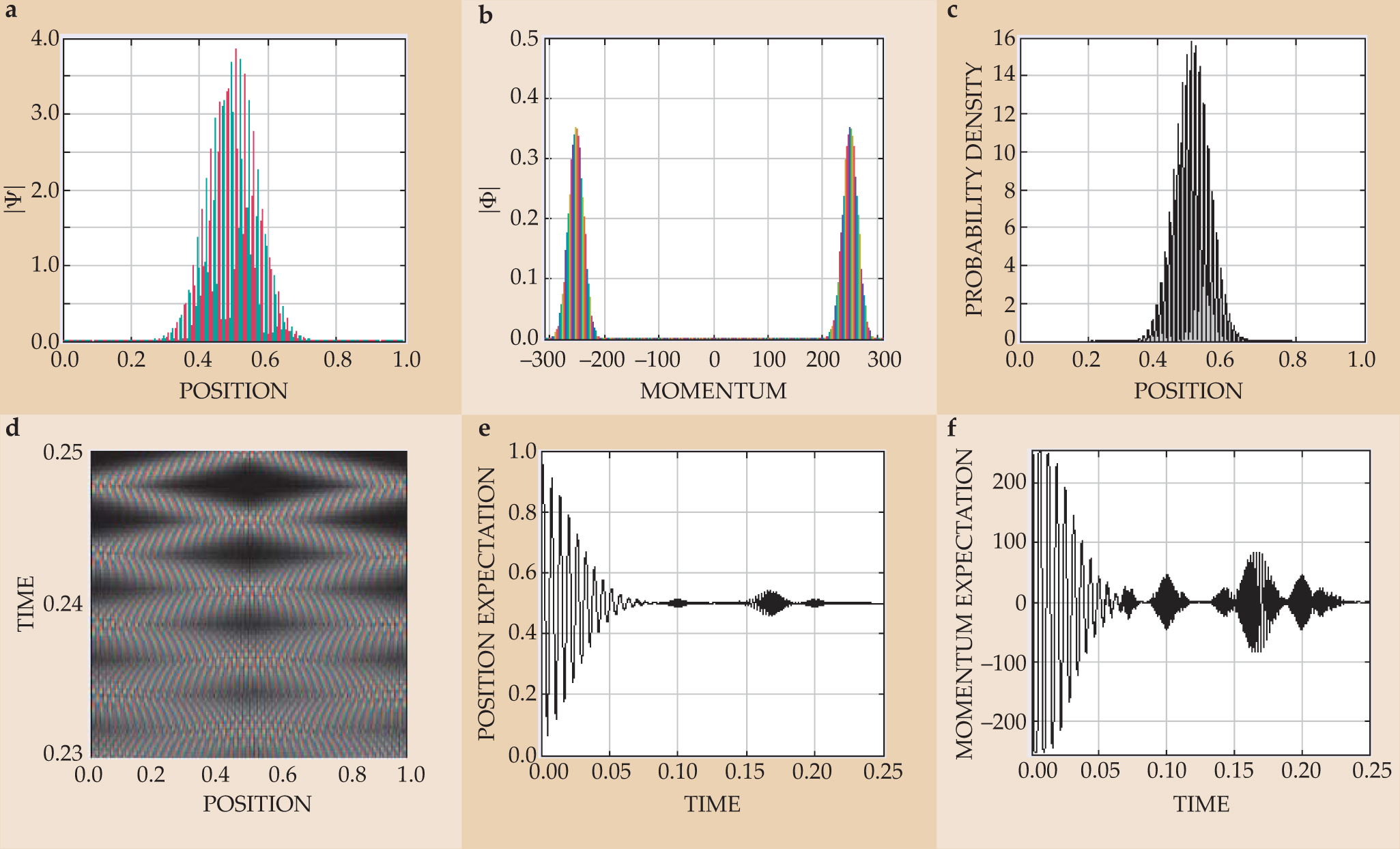
All the quantum mechanics materials developed by the OSP project are accessible via ComPADRE; just go to the Quantum Exchange collection and search under “osp” or “open source physics.” Those resources span the curriculum from introductory subjects to more advanced research-based topics such as the quantum mechanical revivals and fractional revivals that are of current interest to theorists and experimentalists. ¹⁰ Figure 2 shows a fractional revival. It was generated with the OSP QMSuperposition program, which takes the expansion coefficients c_n of a superposition of energy eigenstates ψ_n with energies E_n and evolves the state according to Ψ(x, t) = Σ _n c _n ψ _n (x) exp(–iE_nt)/ħ. That analytic time evolution allows for a fast and accurate depiction of the state even at time scales beyond which numerical solutions often fail.

In addition to classic simulations of quantum mechanical evolution, many computer-based simulations have been developed that cover more contemporary topics, such as quantum information, or foundational issues that are usually skipped in standard sequences. One example is the OSP Spins program, which may be used for focused tutorials such as simulations of single or multiple measurements on spin- $\raisebox{1ex}{$1$}\!\left/ \!\raisebox{-1ex}{$2$}\right.$ particles and even the quantum-mechanical double-slit and other “which-way” experiments. The original Java version of the program was written by David McIntyre, ¹¹ based on an earlier version by Daniel Schroeder and Thomas Moore. The OSP version extends previous work by allowing simulated experiments to be stored and run easily.

Students can gain exposure to various contemporary topics through laboratory experiments. Enrique Galvez and colleagues, for example, have described a set of five experiments in quantum optics that can be set up for about $35 000. ¹² Topics include single-photon self-interference, quantum erasure, and projective quantum measurements. Timothy Havel and coworkers have discussed quantum-information-processing experiments that can be performed using standard and widely available nuclear magnetic resonance spectrometers. ¹³ Laboratory experiences can cement student knowledge and understanding of quantum mechanics and can stimulate students to relate quantum mechanics to things they observe. George Greenstein and Arthur Zajonc’s fascinating book, The Quantum Challenge: Modern Research on the Foundations of Quantum Mechanics (Jones and Bartlett, 1997), suitable for both undergraduates and practicing scientists, is full of descriptions of experiments related to foundations of quantum mechanics and their possible interpretations.

Quantum tutorials

Evidence suggests that the same types of interventions that have proved successful at introductory levels (see, for example, the article by Edward Redish and Richard Steinberg, Physics Today, January 1999, page 24 ) can benefit students of quantum mechanics. In particular, activities that engage students and force them to challenge their beliefs and understandings have the greatest chance of success. Tutorials developed by physics education researchers attempt to bridge the gap between the abstract quantitative formalism of quantum mechanics and the qualitative understanding necessary to explain and predict diverse physical phenomena. They take into account likely student difficulties and provide activities that do not require a total revamping of instructional methods to have an impact. Rather, tutorials can be effective supplements to traditional instruction.

The tutorial approach consists of three main components. First, carefully designed tasks elicit difficulties students have. Then the tutorials guide students through tasks that help them overcome those difficulties and organize their knowledge. The third component is a gradual reduction in tutorial support as students develop self-reliance.

Several features of tutorials make them particularly suited for teaching quantum mechanics.

• ▸ They are based on research in physics education and pay particular attention to cognitive issues.

• ▸ Visualization tools help students build physical intuition about quantum phenomena.

• ▸ Students remain actively engaged as they are asked to predict what should happen in a particular situation and then receive appropriate feedback.

• ▸ Group tutorial activities can supplement lectures, and tutorials can be used outside the class for homework or self-study

• ▸ Self-sufficient modular units can be used in any order.

Daniel Styer ¹⁴ and Dean Zollman and colleagues ¹ have proposed that quantum concepts be introduced much earlier in physics course sequences than is traditional. To assist instructors, Zollman’s group has developed the Visual Quantum Mechanics (VQM) software suite, which is targeted to high-school and college students. ¹⁵ VQM integrates interactive visualizations with inexpensive materials and tutorial worksheets in an activity-based environment. Instructional units include quantum tunneling, luminescence, lasers, and potential energy diagrams. Figure 3 shows an example from VQM in which students explore scattering problems in one dimension. Students can calculate transmission coefficients for 1D scattering potentials, view scattering states, and compute probability densities. One interesting feature of the visualization is that students can change the particle mass or even Planck’s constant and observe the consequences.

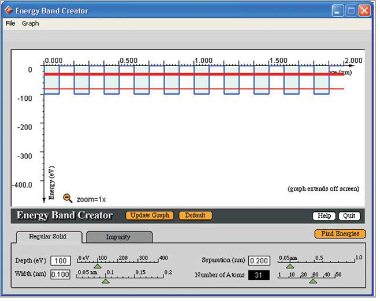
Redish and colleagues have developed a collection of resources incorporating tutorials and visualization tools (including VQM tools and interactive programs called Physlets ⁸ ) to teach modern physics concepts to science and engineering students. ¹⁶ Examples of instructional units include the photoelectric effect, wave–particle duality, spectroscopy, the shape of the wavefunction, light-emitting diodes and quantum mechanical bands, and quantum models of conductivity. In the tutorial dealing with band structure, students are first asked to use a VQM program called the Energy Band Creator to “solve” the time-independent Schrödinger equation for a single finite square-well potential. They then add a second well and observe hybridization or bonding–antibonding states. Finally, they consider a larger number of wells and discover that the allowed energy states form bands. Figure 4 shows an example.

QuILTs

With support from NSF, one of us (Singh) has been developing and evaluating tutorials for upper-level undergraduate and beginning graduate students. The Quantum Interactive Learning Tutorials (QuILTs) have been designed to engage students in the learning process and to help them build links between the abstract formalism and conceptual aspects of quantum mechanics. Topics covered include areas of fundamental and contemporary interest such as the time-dependent and time-independent Schrödinger equations, time development of the wavefunction, the double-slit experiment and which-way information, Larmor precession of spin, and quantum key distribution. QuILTs, which combine conceptual and quantitative problem solving but don’t compromise technical content, are based on the exemplary introductory physics tutorials developed by Lillian McDermott’s group at the University of Washington. ¹⁷

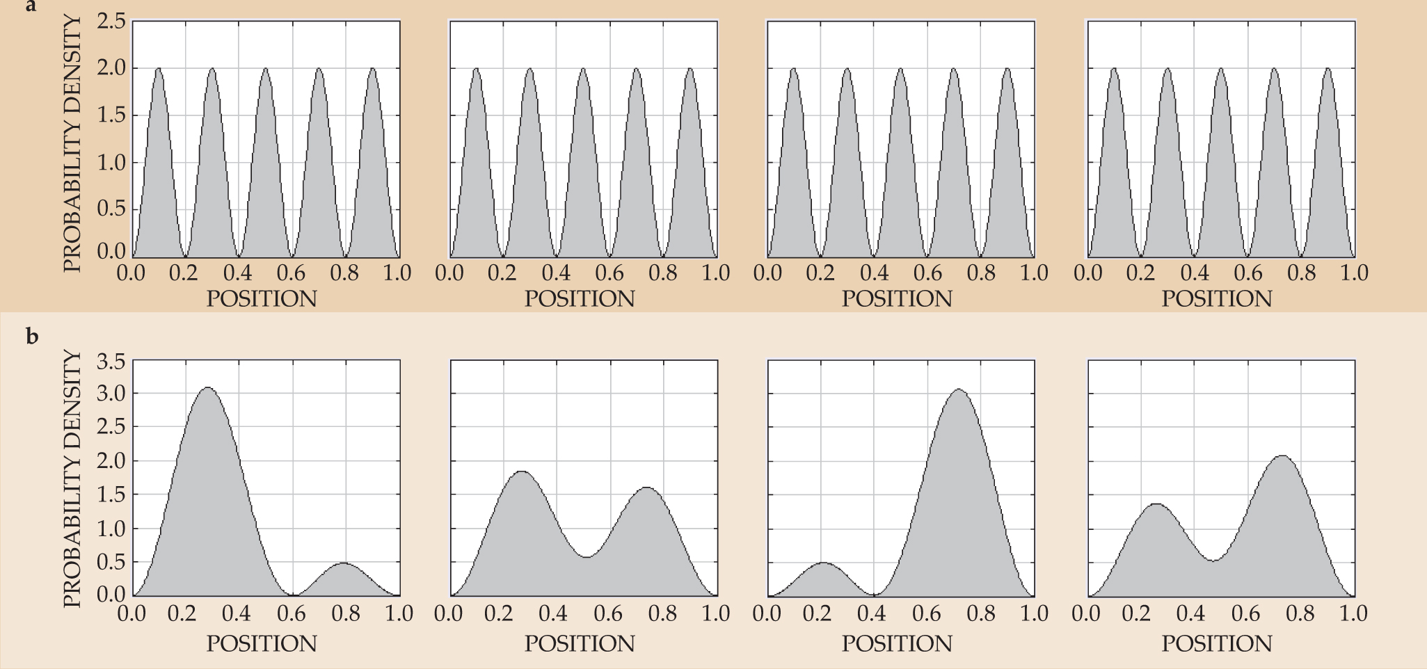
The QuILT dealing with time development begins by asking students to predict the time dependence of two states, one stationary and the other nonstationary, for an electron in an infinite square well. ¹⁸ As discussed earlier, more than half of the students will choose an incorrect answer. The tutorial then asks students to compare their predictions against a computer simulation, adapted from OSP simulations, that gives the evolution of the probability densities for both the stationary and nonstationary cases.

As students see that the probability density does not vary with time for the stationary state (figure 5(a)) but does vary for the nonstationary state (figure 5(b)), they are forced to confront inconsistencies in their thinking. Research on learning suggests that when students reach such a juncture, they want to resolve the discrepancy between their prediction and observation and are highly receptive to guidance that will help them analyze their conceptual difficulties and build a more robust knowledge structure. Working in an interactive environment, students learn by example that the Hamiltonian governs the time evolution of the wavefunction so that the eigenstates of the Hamiltonian are special with regard to time evolution. Moreover, not all allowed states are energy eigenstates. Students must answer questions that relate to concrete examples to help organize their knowledge, and they receive prompt feedback. Then students work on paired problems that use concepts similar to the tutorial problems but for which the contexts are different and help is not provided. The paired problems serve a dual purpose: They help students develop self reliance and provide instructors feedback on the effectiveness of the QuILTs.

The teaching and learning of quantum mechanics currently stand at the fortuitous crossroads where advances in experimental, theoretical, computational, and educational research meet. Physics education research has matured to address courses beyond the introductory level, and in particular researchers have begun to investigate and improve students’ understanding of quantum mechanics. The guidance provided by research-based learning tools has the potential to increase the number and proficiency of students who pursue advanced degrees and careers in physical sciences and engineering.

References

1. See, for example, the theme issue of Am. J. Phys. 70(3) (March 2002) and the papers presented at the 1999 annual meeting of the National Association for Research in Science Teaching, available at http://perg.phys.ksu.edu/papers/narst .
2. H. Fischler, M. Lichtfeldt, Int. J. Sci. Educ. 14, 181 (1992); https://doi.org/10.1080/0950069920140206
P. Jolly et al. Am. J. Phys. 66, 57 (1998) https://doi.org/10.1119/1.18808 .3. C. Singh, Am. J. Phys. 69, 885 (2001); https://doi.org/10.1119/1.1365404
C. Singh, in Proceedings of the 2004 Physics Education Research Conference, J. Marx, P. Heron, S. Franklin, eds., American Institute of Physics, Melville, NY (2005), p. 23;
C. Singh, in Proceedings of the 2005 Physics Education Research Conference, P. Heron, L. McCullough, J. Marx, eds., American Institute of Physics, Melville, NY (2006), p. 69.4. D. Styer, Am. J. Phys. 64, 31 (1996) https://doi.org/10.1119/1.18288 .
5. A. Goldberg, H. M. Schey, J. L. Schwartz, Am. J. Phys. 35, 177 (1967) https://doi.org/10.1119/1.1973991 .
6. S. Brandt, H. Dahmen, The Picture Book of Quantum Mechanics, Springer, New York (2001) https://doi.org/10.1007/978-1-4613-0167-7 .
7. B. Thaller, Visual Quantum Mechanics, Springer, New York (2000).
8. J. Hiller, I. Johnston, D. Styer, Quantum Mechanics Simulations: The Consortium for Upper-Level Physics Software, Wiley, New York (1995);
M. Belloni, W. Christian, A. Cox, Physlet Quantum Physics: An Interactive Introduction, Pearson Prentice Hall, Upper Saddle River, NJ (2006).9. H. Gould, J. Tobochnik, W. Christian, An Introduction to Computer Simulation Methods: Applications to Physical Systems, 3rd ed., Benjamin Cummings, Upper Saddle River, NJ (2006); the Open Source Physics project code library, documentation, and curricular materials can be downloaded from http://www.opensourcephysics.org .
10. H. Katsuki et al. Science 311, 1589 (2006) https://doi.org/10.1126/science.1121240 .
11. See http://www.physics.oregonstate.edu/~mcintyre/ph425/spins/spinsapplet.html .
12. E. J. Galvez et al. Am. J. Phys. 73, 127 (2005) https://doi.org/10.1119/1.1796811 .
13. T. F. Havel et al. Am. J. Phys. 70, 345 (2002) https://doi.org/10.1119/1.1446857 .
14. D. Styer, The Strange World of Quantum Mechanics, Cambridge U. Press, New York (2000).
15. See the Visual Quantum Mechanics website at http://perg.phys.ksu.edu/vqm .
16. E. F. Redish, R. N. Steinberg, M. C. Wittmann, A New Model Course in Applied Quantum Physics, available at http://www.physics.umd.edu/perg/qm/qmcourse/NewModel .
17. L. McDermott, P. Shaffer, Physics Education Group, Tutorials in Introductory Physics, Prentice Hall, Upper Saddle River, NJ (2002).
18. The tutorial can be accessed from http://www.opensourcephysics.org/projects/collections/quilt.html .
More about the authors
Chandralekha Singh is an associate professor of physics and astronomy at the University of Pittsburgh in Pennsylvania. Mario Belloni is an associate professor of physics and Wolfgang Christian the Brown Professor of Physics at Davidson College in Davidson, North Carolina.
Chandralekha Singh, University of Pittsburgh, Pennsylvania, US.
Mario Belloni, Davidson College, Davidson, North Carolina, US.
Wolfgang Christian, Davidson College, Davidson, North Carolina, US.