Branched flow

Small causes can have large downstream effects. That idea is the foundation of chaos theory. But chaos needs time and space to develop, and fascinating behavior can happen on the way. As a directed wave or a collection of rays, such as light, travels through an almost homogeneous medium, even minute random variations in the medium can lead the wave and the rays to branch off and cause extreme intensity fluctuations. That phenomenon is known as branched flow. Examples include the height fluctuations of tsunamis, the flow of electrons in semiconductors, and pulsar radiation propagating through the interstellar medium. This article gives an overview of branched flow, its prerequisites and implications, the breadth of systems in which it has been observed, and the reasons it’s so ubiquitous. And the journey to understanding this intriguing phenomenon has just begun.

Branched flow occurs whenever waves travel through complex environments that can be characterized by random, spatially smooth, and modest variations in the refractive index or its analogue. The characteristic spatial scales of the variations (their correlation lengths) must exceed the wavelengths, and their magnitudes must be small enough that the waves or rays representing them are only weakly deflected. In other words, the waves are only forward scattered. Those conditions are frequently met in natural and technological environments. Sound, light, vibrations, and water waves are all dramatically affected by branched flow.

The phenomenon of branched flow shows up in electron waves when they are refracted by residual disorder in high-mobility semiconductors and by deformation potentials in pure metals and semimetals. It emerges in ocean waves deflected by surface eddies in the sea currents; in sound waves refracted in the turbulent atmosphere and refracted underwater by variations in temperature, salinity, and pressure; and in tsunami waves refracted by variations in the ocean’s depth. Light undergoes branched flow when it experiences gravitational lensing by galaxy clusters and their associated dark matter, when it is deflected in media with refractive index fluctuations, and when it is refracted by living tissue. Branched flow is even responsible for the voids and filaments in the structure of the universe.

The behavior has been hiding in plain sight in those and many other physical phenomena. But now awareness of branched flow and its importance is rapidly expanding. The increasing understanding that diverse physical systems with wildly different length scales can reflect similar mathematics and physics is benefiting a wide array of disciplines.

Why is the study of such a ubiquitous and important phenomenon just now getting under way? A likely answer is the lack of computers in the past and physicists’ initially slow adoption of computer graphics. Without that computing power, the focus was on analytical theories, which are most feasible at the two extreme ends of the branched-flow problem: the first random focusing events and the final regime of diffusive statistical mixing. Between those extremes lies the ballistic domain of branched flow. The mathematics of that domain remain underdeveloped, and graphical discoveries and computer simulations are essential to present and future development.

Tsunami waves

Perhaps the most terrifying example of branched flow, ocean tsunami waves are a good platform to introduce the phenomenon. Subsurface earthquakes and large coastal landslides can excite highly energetic surface ocean waves with long wavelengths from tens to hundreds of kilometers. The waves travel hundreds of kilometers an hour in shallow water relative to their wavelengths.

The March 2011 magnitude 9 earthquake off the coast of Tohoku, Japan, for example, sent waves propagating out like ripples. For the waves heading away from shore, weak refraction caused by variations in ocean depth accumulated to create dramatic wave height variations in a branched shape, as illustrated in the NOAA tsunami reconstruction in figure 1. That image is typical of branched flow. (To see additional images, including an informative animation, visit https://nctr.pmel.noaa.gov/honshu20110311 .)

Figure 1.

The speed of the tsunami wave is proportional to the square root of the ocean depth, averaged over scales on the order of the wavelength. Underwater mounds act as focusing lenses, ¹ and depressions act as diffusing lenses. Even depth fluctuations of only a few percent can lead to the formation of branches. Unfortunately, the bottom depths of Earth’s oceans are not known well enough to accurately predict the locations of distant tsunami branches. ² If the ocean depths were better known, life-saving predictions could be taken well before destructive energy reached shore.

Because branched flow results from many random small-angle refraction events caused by smooth weak inhomogeneities, such as ocean depth variations, that span more than one wavelength, classical ray tracing applies. For branched flow to occur, the source of the waves needs to be at least weakly localized, such that it can be described as a surface or manifold in phase space. To understand why, imagine how clearly a lens focuses sunlight on a sunny day, when the rays of the Sun are almost parallel, compared with the hard-to-see focus on a cloudy day with diffuse lighting. Examples of localized sources include emission in many directions from a spatially localized point, such as the waves from the Tohoku earthquake and radio waves from a pulsar, and a spatially extended source with restricted initial propagation directions, such as a plane wave (see the box on page 49).

First steps in branched flows

Branched flow is the spatial pattern that forms when a wave or a bundle of rays is launched over a smooth, weakly refracting random potential. The pattern begins (but doesn’t end) with singularities called cusps, shown here. In optics, such singularities are called caustics and typically result from refraction or reflection by curved surfaces. ²¹ Along caustics, the number of ray solutions passing through a point in coordinate space changes abruptly.

In the top left panel, the rays pass from left to right perpendicular to a concavely curved surface (bold black curve). The result is an imperfect focus: a cusp caustic from which two fold caustics sprout (see the middle left panel). The geometry resembles that of a folded sheet.

The bottom left panel shows how initially parallel trajectories (thin black lines) are weakly deflected by the potential indicated by a blue-scale color map in the background. The white lines show successive phase-space representations ($y$ versus $v_y$) of the ray bundle. Although for short times only one ray solution passes through every $y$, after the cusp point a region emerges in which the white line traverses each point three times.

The top and middle left panels show that the projection of the phase-space manifold on to real space leads to singularities in ray density. On the right, an initially parallel bundle of trajectories with total energy $E$ traverses along the $x$-axis over a correlated random potential $U(x,y)$ with mean $⟨U⟩=0$ and standard deviation $\sqrt{⟨U^2⟩}=ϵ=0.01E$.

Many natural sources correspond to fuzzy manifolds that are only semilocalized in phase space; examples include light rays from the Sun and waves leaving a storm in one region of the ocean in a range of directions. The branching phenomenon is still rich and dramatic for those averaged sources.

Ray modeling

The simulations in figure 2 show ray (green) and wave (purple) intensities emitted from a central point source over the same smoothly varying weak random potential. The two solutions have some obvious agreements and some subtle differences. Although the gross branched structures agree, wave interference effects are prominent for coherent sources, such as the frequency-sorted pulsar radio waves arriving at Earth. At long propagation distances, the differences between ray simulations and the actual wave evolution can be profound.

Figure 2.

In the opening image, the same ray-tracing simulation is extended to follow more generations of fold catastrophes. It possesses striking stable branches, which result in strong flux density indicated by the darkest curving lines. To track the phase-space characteristics of classical flow, one can draw a surface (in figure 2, the circle) perpendicular to the average flow and plot each ray’s position (here the angle $\phi$) of intersection as a function of its momentum component $p_{\phi }$ along that so-called Poincaré surface of section. The intersection (black curves in the figure) reveals how the flow evolves in phase space and indicates when lines fold over, a phenomenon known as caustics. The evolution is equivalent to an area-preserving mapping of the phase plane onto itself.

Photoshop dynamics

A discrete-time nonlinear ray map, known as kick and drift, is a quick and instructive way to reveal branched flow’s essence, causes, and effects. The kick–drift ray map replaces propagation across a random potential with a succession of independent and random refractive thin lenses separated by regions in which the wave can flow freely.

To create your own, use Photoshop (or our python script at https://github.com/tobiaskramer/branch ) and start with a phase plane $(x,p_x)$ with fuzzy manifolds marked by colored bands that span a small range of initial momenta, as shown in frame 1 of figure 3. Then apply a random area-preserving momentum kick (Filter:Distort:Wave in Photoshop; set the horizontal scale to a minimum), which causes vertical undulations in the manifolds, shown in frame 2. You can adjust the amplitude, number of generators (sines are best), and the wavelength range of the sines by experimentation. (Be careful: You might discover a new regime!) Next, apply an area-preserving drift step (Filter:Distort:Shear), which leads the different momenta from the first step to cause shearing; that step is free-particle drift, shown in frame 3. You can adjust the amount of shearing. Next, repeat that two-step cycle with a random and independent kick–drift, as in frame 4. Just a few iterations lead to frame 5, shown magnified in frame 6.

Figure 3.

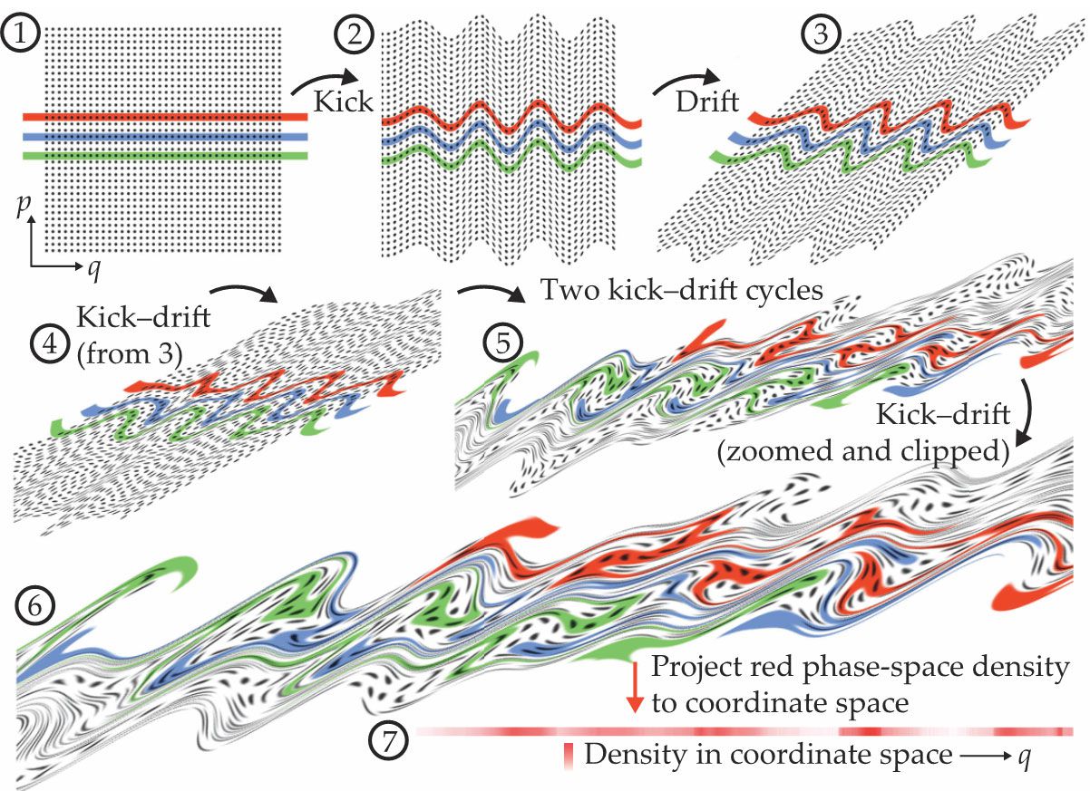
You can see thickening of the manifold in some regions and thinning in others, even as it is stretched in overall length. Some stable or nearly stable zones survive the six kick–drift cycles, as indicated by the black disks that are still relatively undistorted in frame 6. The points in the red fuzzy manifold end up nonuniformly distributed in position $(x)$ space, as shown in the projection onto coordinate space in frame 7. The red clusters in that projection correspond to branches similar to those in the opening image.

The kick–drift model is equivalent to the small-angle approximation for a series of thin lenses in the optical case. Most zones in frame 7 have contributions from more than one red region in the phase plane. In the wave or quantum version, those separate contributions would carry their own phase and amplitude and interfere constructively or destructively with one another. The qualitative features here apply even after thousands of kick–drift cycles.

The kick–drift model can be defined as a simple point-to-point area-preserving mapping of the phase plane onto itself, under $$p_{n+1}=p_n-{\overline{)\frac{d{V}_n(x)}{dx}}}_{x=x_n}\text{(kick step) and}$$ $$q_{n+1}=q_n+p_{n+1}\text{(drift step).}$$

The potential $V_n(x)$ changes randomly with each iteration $n$, although it retains certain statistical properties, such as a correlation length in $x$.

Dimensionality

The branching phenomenon applies in both two- and three-dimensional wave flow. Figure 4 is a ray-tracing simulation of 3D propagation similar to what might occur for sound waves refracting in an atmosphere with temperature and velocity fluctuations.

Figure 4.

A common real-world example is the irregular variations in the volume of a jet aircraft overhead. They occur because the loudness pattern on the ground, akin to the light pattern at the bottom of a pool, moves as the jet moves. Indeed, the chance that atmospheric focusing of damaging sonic booms could affect such sensitive places as operating rooms contributed to the 1971 ban of commercial supersonic flight over land in the US.

Characteristic length scales

In figure 2, what determines the average distance between the first focal cusps along the angular direction and the average radial distance $L$ from the origin to the first cusps? ³ For classical flow of energy $E$ traveling over smooth potential undulations of typical height or depth $ϵ\ll E$, the distance between cusps is $L\propto d{(E/ϵ)}^{2/3}$ in terms of the correlation length $d$ of the potential bumps.

That and other statistical properties of the branched flow are largely independent of the details of the random potential and are thus as universal as the concept of a mean free path. ⁴ Over an ensemble of random potentials, the momentum starts as a delta peak at $\phi =0$ and then diffuses as $$P(\phi ,t)=\frac{1}{\sqrt{4\pi Dt}}{e}^{-\frac{{\phi }^2}{4Dt}}\text{,}$$ with $D\propto {ϵ}^2/E^{3/2}d$. The direction of travel decays as $$\int P(\phi ,t)\cos (\phi )d\phi =e^{-t/\tau }\text{,}$$ where $\tau =1/D$.

To have branched flow in a system, its dimensions must be smaller than the mean free path, or, at least, the observation time must be shorter than the mean free time. Beyond the mean free path, rays will start to turn around, and their propagation will no longer be ballistic but diffusive. But in weakly refracting media, when $ϵ/E\ll 1$, the mean free path $l=⟨|v|⟩\tau \propto {(ϵ/E)}^{-2}d$ is much larger than the typical branching length scale, which scales like ${(ϵ/E)}^{-2/3}$. Thus for a wide regime, wave propagation is dominated by branched flow.

As mentioned earlier, branched flow has two other prerequisites. First, the source needs to be restricted in phase space—for example, a point, parallel ray, or plane wave. Sources with fuzzy but still somewhat localized manifolds, however, also produce pronounced branched flows and lead to extreme events. The second prerequisite is that the flows’ wavelength needs to be smaller than the correlation length of the random medium.

Stable branches

More study is needed to elucidate the geometry of classical ray-tracing branched flow, the geometry of wave-propagation branched flow, and the relation between them. For example, caustics—phase-space fold catastrophes projected onto coordinate space—do not alone account for the formation of strong branches. Another contributing factor is quantified by the rarefaction exponent, a measure of the stretching or compression of the initial manifold tangential to the manifold surface. ⁵ Compression along that direction can pile up flux density and create branches without caustics or enhance branches with them.

In one of the first numerical studies of the branched flow of sound in the ocean, Michael Wolfson and Steven Tomsovic of Washington State University in Pullman recognized a stable subclass of branches: zones of initial conditions in which trajectories coincidentally remain nearby one another for some finite distance or time. ⁶ For some initial conditions, successive dilations and contractions of phase space almost temporarily cancel each other. The odds of such lucky initial conditions decrease exponentially with time, but some nearly stable zones continue to exist. Examples of nearly stable zones are the relatively undistorted disks in figure 3 that survived six violent kick–drift steps and the ray bundles in the opening image.

Structure of the universe

Caustics and folds contribute to the distribution of matter in the universe. The popular Zeldovich model of the large-scale structure of the universe proposes that the universe resulted from a single kick–drift episode, followed by sticky gravitational effects after caustics formed. According to the model, the relatively uniform distribution of the matter in the early universe possessed random fluctuations in velocities down to some cutoff length scale. (An alternative explanation is that the initial dynamics resulted from a slow gravitational acceleration because of nascent mass-density fluctuations.)

Both mass and velocity variances could arise from quantum fluctuations in the first moments of the universe. Cases with mass, velocity, and combined mass and velocity variations include a long period of free or weakly accelerated drift of relatively tenuous and mostly noninteracting matter. That kick–drift cycle leads to the formation of caustics, which resemble those in figure 4b, before gravitational effects change the dynamics. Numerical simulations based on those ideas give rise to structures similar to the observed cosmic web of matter, including the large voids, ⁷ as highlighted in the “Caustics and pancakes” section of James Peebles’s classic 1980 textbook The Large-Scale Structure of the Universe.

The initial kick–drift episode is analogous to sunlight falling on a pool bottom after being refracted just once by surface waves. How matter flies off the undulating surface of a comet is much the same story: Matter is ejected mostly in the normal direction from every point on the comet’s surface. ⁸

Pulsar radio waves

A similar model applies to radio waves emitted by pulsars. As the waves make their way to Earth, one or more partially ionized interstellar clouds often refract them. Between clouds, the waves propagate in long expanses of free space until finally reaching Earth. The radio source is ideal for observations: pulsed, broadband across frequencies $\omega$, and a virtual pinpoint in the sky. The ionized clouds disperse the waves with propagation speed proportional to $1/{\omega }^2$ and total time delays that scale with the total density of electrons in the wave’s path. For a typical pulsar at 1 kpc distance from Earth, microwaves take several minutes or more to arrive, with the shortest wavelengths arriving at Earth first. The refractive index in a cloud likely varies at many different scales.

Instruments installed at radio telescopes, such as the Arecibo Observatory in Puerto Rico, process data to produce what’s known as a spectrogram. Such measurements track the signal strength as a function of time, typically on the order of hours, and frequency, typically a snapshot of a 10 MHz interval between 30 and 1500 MHz, well within uncertainty principle limits.

Besides the characteristic pulsations, whose periods lie mostly in the range 0.1 to 10 seconds, a typical signal varies dramatically by the day, hour, and minute at a single telescope. That variation results from a combination of the pulsar moving relative to a cloud, Earth presumably passing through different branches, and the interference of coherent microwaves that have taken different paths to reach the telescope.

Pulsar radio waves are the earliest example that we (the authors of this article) could find of ray tracing leading to a clear depiction of the branched-flow regime, as shown in figure 5a. Alexander Pidwerbetsky introduced the technique in his 1988 dissertation, ⁹ which built on his seminal pulsar paper with James Cordes and Richard Lovelace. ¹⁰

Figure 5.

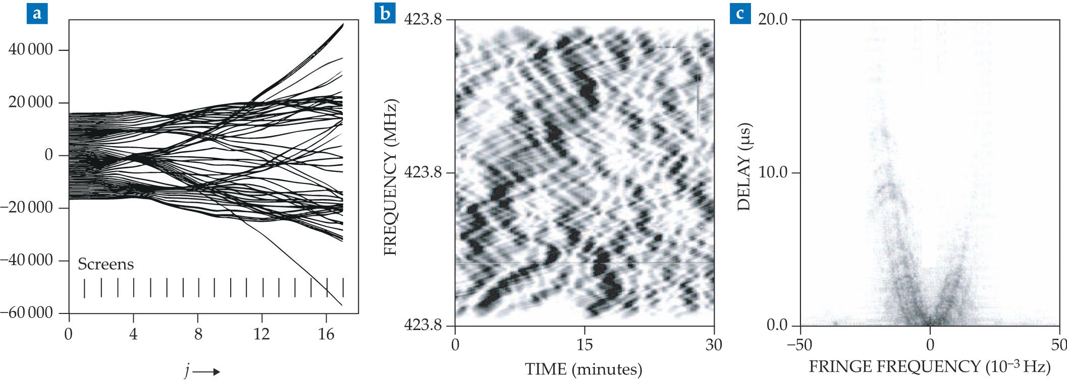
A recent innovation uses a double Fourier transform of the radio telescope time–frequency dynamic spectrum, or primary spectrogram, to create a secondary spectrum, or Fourier spectrogram. ¹¹ The results look nothing like the primary spectrum, shown in figure 5b, and contain information about the properties of the interstellar clouds, such as their locations, structures, and densities. They often feature one or two sometimes sharp parabolic arcs, characteristic of each pulsar, as shown in figure 5c.

The clouds are modeled as thin sheets and can generate something akin to kick–drift dynamics for several successive cloud encounters. As early as 1986, Cordes and Aleksander Wolszczan noted, “multipath refractive scattering must be a common occurrence” in pulsar microwaves arriving at Earth. ¹² That is, they identified branched flow.

The pulsar data are so rich that they inspired new laboratory measurements on other systems—in particular, experiments with broadband and pulsed point sources and detectors with time scales shorter than those in the medium. Such probes are well suited for measuring turbulence.

Semiconductors and pure metals

We first encountered branched flow in micrometer-scale scanning-probe-microscope measurements of electron flow in 2D electron gases (2DEGs). About 20 years ago, Robert Westervelt’s lab at Harvard University produced spectacular images of that electron flow by mapping out the variations in transmission through the 2DEG. Those images include high-resolution ones showing interference fringes in the scattered electron waves. ^{13 , 14} (See the article by Mark Topinka, Bob Westervelt, and Rick Heller, Physics Today, December 2003, page 47 .) Theoretical models of a typical potential field experienced by an electron in a 2DEG revealed the origin of the branched flow in those experiments. ¹⁴ Adjacent ionized atoms supply electrons to the 2D layer and induce a smooth nonuniform potential field that randomly deflects the electrons flowing through a small opening between two electrodes, known as a quantum point contact.

Recently, researchers established theoretically that branched flow governs electrical resistivity in pure metals and semimetals from 0 K up to room temperature and often beyond. At finite temperatures, lattice vibrations in a material cause strain and a resulting deformation potential. The researchers treated that deformation potential as exerting a classical force on the conduction electrons. Previously, the deformation potential had been included only in the context of first-order, single-phonon quantum perturbation theory. The electrons could change directions and thus cause scattering and resistivity only by creating or annihilating a quantized lattice vibration, or phonon. We treated successive scatterings with the Boltzmann equation.

The transition from a low-temperature $T^4$ rise in resistivity in 2D systems and a $T^5$ in 3D ones to a $T^1$ rise at high temperatures was seen numerically and analytically using branched-flow trajectories. Classical perturbation theory finds the same expressions, including prefactors, for the resistivity as quantum perturbation theory. The branched-flow description introduces a new picture of electrons colliding with moving potential bumps, which exchange momentum and energy, and the ability to go beyond the perturbative regime. That picture, illustrated in figure 6, captures what is really going on rather than just statistical measures.

Figure 6.

Freak waves and soap bubbles

Shortly after the 2DEG electron flow data were understood to result from branched flow, the search began for other wave phenomena that might experience a branched-flow regime. That search revealed that branched flow is a universal wave phenomenon. An important example is the propagation of a storm’s wave energy through random refracting current eddies in the ocean. With one exception, the field of extreme ocean waves had made a jump from a theory of uniform sampling Gaussian random statistics, developed by Michael Longuet-Higgins in the 1950s, to considerations of nonlinear wave interactions. The impetus for that jump was the field observations, starting in the 1990s, of far more freak wave events than accounted for in uniform Gaussian random statistics.

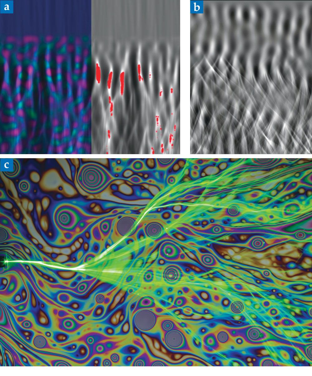
Benjamin White of Exxon Research in New Jersey and Bengt Fornberg of the University of Colorado Boulder were the exception; they attributed freak waves to focusing by gyres. Their 1998 study using a simple incident plane wave gave a clear early example of caustics and branched flow. ¹⁵ But they did not consider dispersion in the initial wave propagation direction—in other words, they used a sharp initial manifold rather than a more realistic fuzzy one. Critics in the field argued that fuzziness would wash out the effects of caustics. Subsequent work showed that initial dispersion does not wipe out even large wave energy fluctuations downstream. In fact, the branching develops more contrast and even finer structure downstream (see figures 7a and 7b).

Figure 7.

Schemes that include those fluctuations in nonuniform Gaussian sampling predict a factor of 50 more freak wave events than those with uniform sampling; no nonlinear wave interactions are required. ¹⁶ (Nonlinear effects are, however, important in the formation of the largest waves. ¹⁷ )

The connection between branched flow and freak ocean waves has inspired studies of freak-wave formation in microwave cavities ¹⁸ and of methods for selectively populating optical branches. ¹⁹ Visible light injected into a soap bubble film can also undergo branched flow if the variations in the bubble-film thickness are random and correlated. Figure 7c shows an image from one such experiment. ²⁰

Branched flow emerges everywhere. It lies in the interesting regime between the first focal cusps and eventual random diffusive scattering. The universality of the phenomenon and the huge range of applications at astronomically different scales, from nanometers to the whole universe, suggest branched flow is worthy of further investigation with numerical, experimental, and, especially, mathematical characterizations.

References

1. M. V. Berry, Proc. R. Soc. A 463, 3055 (2007). https://doi.org/10.1098/rspa.2007.0051
2. H. Degueldre et al., Nat. Phys. 12, 259 (2016). https://doi.org/10.1038/nphys3557
3. V. A. Kulkarny, B. S. White, Phys. Fluids 25, 1770 (1982); https://doi.org/10.1063/1.863654
L. Kaplan, Phys. Rev. Lett. 89, 184103 (2002). https://doi.org/10.1103/PhysRevLett.89.1841034. J. J. Metzger, R. Fleischmann, T. Geisel, Phys. Rev. Lett. 105, 020601 (2010); https://doi.org/10.1103/PhysRevLett.105.020601
J. J. Metzger, R. Fleischmann, T. Geisel, Phys. Rev. Lett. 112, 203903 (2014). https://doi.org/10.1103/PhysRevLett.112.2039035. E. J. Heller, S. Shaw, Int. J. Mod. Phys. B 17, 3977 (2003). https://doi.org/10.1142/S0217979203021964
6. M. A. Wolfson, S. Tomsovic, J. Acoust. Soc. Am. 109, 2693 (2001). https://doi.org/10.1121/1.1362685
7. S. N. Gurbatov, A. I. Saichev, S. F. Shandarin, Phys.-Usp. 55, 223 (2012). https://doi.org/10.3367/UFNe.0182.201203a.0233
8. T. Kramer et al., Adv. Phys.: X 3, 1404436 (2018). https://doi.org/10.1080/23746149.2017.1404436
9. A. Pidwerbetsky, “Simulation and analysis of wave propagation through random media,” PhD thesis, Cornell U. (1988).
10. J. M. Cordes, A. Pidwerbetsky, R. V. E. Lovelace, Astrophys. J. 310, 737 (1986). https://doi.org/10.1086/164728
11. D. R. Stinebring, Chin. J. Astron. Astrophys. 6, 204 (2006). https://doi.org/10.1088/1009-9271/6/S2/38
12. J. M. Cordes, A. Wolszczan, Astrophys. J. 307, L27 (1986), p. L30. https://doi.org/10.1086/184722
13. K. E. Aidala et al., Nat. Phys. 3, 464 (2007). https://doi.org/10.1038/nphys628
14. M. A. Topinka et al., Nature 410, 183 (2001). https://doi.org/10.1038/35065553
15. B. S. White, B. Fornberg, J. Fluid Mech. 355, 113 (1998). https://doi.org/10.1017/S0022112097007751
16. E. J. Heller, L. Kaplan, A. Dahlen, J. Geophys. Res. Oceans 113, C09023 (2008). https://doi.org/10.1029/2008JC004748
17. L. H. Ying et al., Nonlinearity 24, R67 (2011); https://doi.org/10.1088/0951-7715/24/11/R01
G. Green, R. Fleischmann, New J. Phys. 21, 083020 (2019). https://doi.org/10.1088/1367-2630/ab319b18. R. Höhmann et al., Phys. Rev. Lett. 104, 093901 (2010).; https://doi.org/10.1103/PhysRevLett.104.093901
S. Barkhofen et al., Phys. Rev. Lett. 111, 183902 (2013). https://doi.org/10.1103/PhysRevLett.111.18390219. A. Brandstötter et al., Proc. Natl. Acad. Sci. USA 116, 13260 (2019). https://doi.org/10.1073/pnas.1905217116
20. A. Patsyk et al., Nature 583, 60 (2020). https://doi.org/10.1038/s41586-020-2376-8
21. M. V. Berry, C. Upstill, in Progress in Optics, vol. 18, E. Wolf, ed., North Holland (1980), p. 257;
J. F. Nye, Natural Focusing and Fine Structure of Light: Caustics and Wave Dislocations, IOP (1999).
More about the authors
Eric Heller is a professor in the departments of physics and of chemistry and chemical biology at Harvard University in Cambridge, Massachusetts. Ragnar Fleischmann is a scientist at the Max Planck Institute for Dynamics and Self-Organization in Göttingen, Germany. Tobias Kramer is a professor of theoretical physics at Johannes Kepler University Linz in Austria.