Bone, implants, and their interfaces

Each year in the US, between 1 million and 2 million dental implants and some 600 000 artificial hips and knees are placed. Those numbers will almost certainly grow: Demand for joint replacements is predicted to increase by 175% over the next 15 years. Although the vast majority of the procedures are successes, about 5–10% of dental implants fail in service and nearly 7% of all joint replacements are revision surgeries to replace a previous, failed implant. Often, the failures can be attributed to poor bonding between the bone and the implant.

Several factors determine how well an implant will bond with native bone. They include physical and chemical factors, such as the chemical composition, porosity, and surface morphology of the implant, and patient-specific factors, such as age, bone quality, and overall health. The patient-specific factors often aren’t controllable. Still, a better understanding of how biomaterials integrate with bone can lead to improved device materials and fewer device failures.

On that front, the biomaterials research community has already made great strides. Since the discovery in the 1960s that bone can adhere to nonbiological materials—a phenomenon known as osseointegration—our understanding of the behavior has improved considerably, and so has the design of implant materials and devices. Yet an important question remains unanswered: At what structural length scale does bone–implant bonding actually occur?

Several research groups are pursuing the answer to that question. They are aided by state-of-the-art three-dimensional imaging techniques that assess bone–implant bonding from the microscale to the nanoscale. In this article I’ll review those techniques and explore how they’re helping to unlock the mysteries of osseointegration.

An intricate hierarchy

At the macroscopic scale, our long bones—femurs, clavicles, tibiae, and the like—are composite materials: A dense outer shell, made of so-called compact bone, surrounds a sponge-like interior known as trabecular bone. The unique structural combination optimizes the distribution of stress and maximizes the bone’s strength-to-mass ratio.

Perhaps more interesting than bone’s macrostructure, however, is its dynamic nature. Bone cells can respond to applied stresses by remodeling the bone’s structure to better withstand regular loading cycles. That’s what causes the bone in a tennis player’s dominant forearm to grow thicker over time and, conversely, the bones of an astronaut to lose mass in microgravity. Bone’s dynamic nature also helps it heal: Throughout a typical person’s healthy lifetime, numerous microfractures will be identified, removed, and replaced as a result of the interplay between bone cells. In fact, up to 10% of our bone mass turns over every year, which makes bone arguably one of the most actively self-healing materials in the world. Rich in calcium, phosphorous, and sodium, bone is also our bodies’ largest ion reservoir and, as such, plays an important role in maintaining homeostasis.

At micro- and nanoscales, bone reveals a complex hierarchical structure that has distinct levels of organization, illustrated in figure 1. Nine levels in total have been classified. (For detailed discussions of all of them, see reference and the article by Rob Ritchie, Markus Buehler, and Paul Hansma in Physics Today, June 2009, page 41 .) At the simplest level, bone is approximately 35% collagen protein and 65% hydroxyapatite, a natural mineral rich in calcium and phosphate. Bone also contains water and noncollagenous proteins.

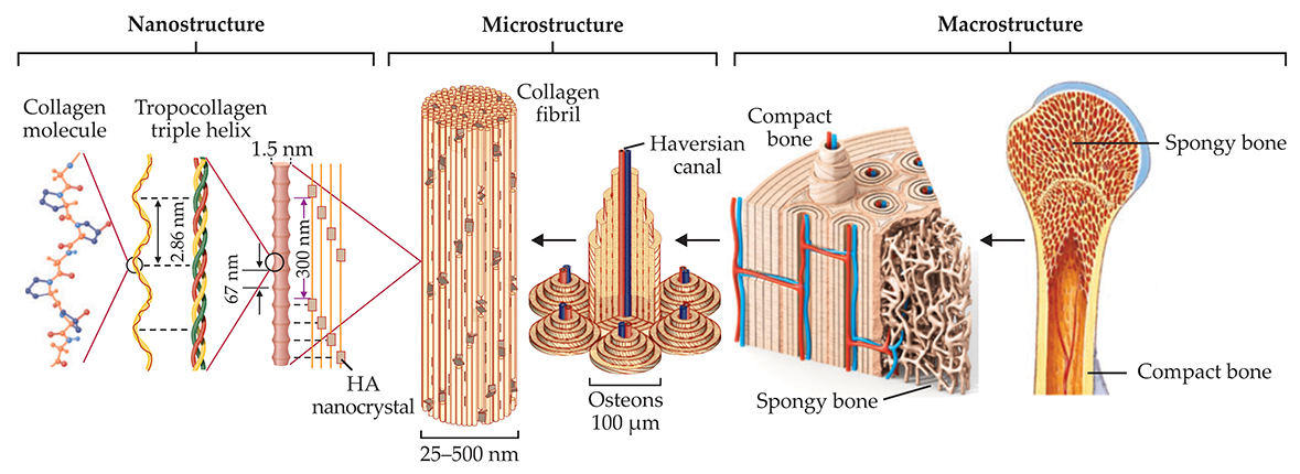
The collagen molecules maintain a unique relationship among themselves: They organize into fibrils, with alternating overlap and gap regions having a periodicity of about 67 nm. (That periodicity is common across many species and many types of collagenous tissue, not just bone.) Nanocrystals of hydroxyapatite position themselves inside the gaps with their c-axes—their long axes—aligned with the length of the fibril. That small-scale organization contributes to bone’s large-scale fracture toughness. Recent studies suggest that hydroxyapatite can also be found in the space between fibrils. The mineralized collagen fibrils serve as building blocks for higher-level architectures such as the concentric osteons that make up the majority of our compact bone. ²

How bones bond

The discovery of bone–metal bonding happened by accident. In the 1960s Per-Ingvar Brånemark was using a titanium chamber to view blood flow in rabbits when he found it extremely difficult to remove the titanium from bone. Brånemark coined the term osseointegration and went on to develop one of the most widely used dental implant systems of the present day. ³ Titanium remains a popular biomaterial for load-bearing bone implants due to the biocompatibility of its naturally bioinert titania surface layer.

Bones don’t bond with nonbiological materials in the traditional sense; that is, the materials aren’t held together by simple ionic or covalent chemical bonds. Rather, osseointegration is a complex multimechanistic event influenced and mediated by several biological factors. ⁴ In the simplest picture, illustrated in figure 2, the process begins when proteins adhere to the implant surface and initiate a cascade that results in the recruitment of bone cells to the interface. Those cells deposit extracellular matrix known as osteoid, which mineralizes into bone. Because it forms so rapidly, that initial, so-called woven bone tends to be structurally disorganized. With time, it remodels itself into the more hierarchically structured bone described above. ⁵

Interestingly, small changes in the porosity and surface topography of an implant can have a profound effect on the strength of the bone–implant bond. The implant’s chemical makeup and biocompatibility are also important: For instance, hydroxyapatite and calcium phosphates tend to work well because they are chemically similar to natural bone, and titanium is popular because of its bioinert surface layer. But studies suggest that even relatively small changes in an implant’s surface topography can improve the outcomes of replacement surgeries. ⁶ If an implant has pores roughly 100 µm or larger, for instance, new bone can grow into those pores, mechanically interlock with the implant surface, and thus enhance the degree of fixation.

Recent work has established that fixation can be further enhanced by combining microscale porosity with nanoscale roughening. Such multimodal surface structure optimizes the cellular and in vivo response to implantation: A partial 30% increase in an implant’s nanoscale surface roughening can produce up to a 150% increase in biomechanical stability, quantified by the force required to extract the implant. Advances in surface design can have huge clinical implications: Next-generation porous titanium cups, for instance, are enabling surgeons to perform hip replacements where previously there wasn’t enough bone to achieve fixation.

Osseointegration has also benefited considerably from improvements in coatings. In particular, hydroxyapatite coatings, often applied by a plasma-spraying technique, offer a dual advantage: They enhance the nanotopography of the bone–implant interface, and they provide a surface that is chemically similar to bone tissue. Future coatings, however, will need to do more than just improve osseointegration; also important will be mitigating the patient’s foreign-body response and risk of infection. ⁷ With those factors in mind, next-generation implant coatings are being designed to incorporate antibacterial and antibiotic elements, such as silver nanoparticles, locally released drugs, and macromolecules that initiate a desired gene response.

In recent decades biomaterials researchers have begun pursuing an alternative to replacement: endogenous regeneration, in which the implanted device is made of so-called resorbable materials that promote the natural healing and regrowth of the native tissue. Ideally, the implant is gradually replaced by the regenerating native tissue.

Resorbable materials include ceramics such as some calcium phosphates, polymers such as poly-caprolactone, and composites of the two. One well-known example is bioglass, a widely used, bioactive glass–ceramic composite developed in the 1960s. ⁸ Like implant coatings, resorbable biomaterials can be augmented with growth factors, including bone morphogenetic protein, and with other biomolecules that modulate natural healing processes in the body. Some researchers envision using in vivo bioreactors in cell-rich regions of the body to generate new tissue that can then be transplanted to the sites where it’s needed. ⁹ Other, as yet undiscovered approaches to regenerative medicine could revolutionize our approach to implant design in the near future.

As of now, however, permanent implant devices such as titanium and stainless steel still have a place in biomaterials, particularly in load-bearing applications. And there’s room to improve them. To do so, however, we’ll need an intimate understanding of the processes that bond bone at the smallest length scales. And for that, we’ll need imaging techniques ranging from the macroscale to the nanoscale and beyond.

Imaging with photons

When osseointegration was discovered in the 1960s, 2D light microscopy was the gold standard in characterization. Using a technique known as histology, one can stain a specimen with a chemically selective dye and obtain clues to biological events. A number of seminal observations on bone structure and bone–implant bonding were made using light microscopy and other 2D imaging and spectroscopic techniques, such as Raman and IR spectroscopy, small-angle x-ray scattering, and transmission electron microscopy (TEM). Many of those 2D imaging approaches are still widely used today.

Due to both the inhomogeneity of the bone tissue near an implant interface and the complexity of today’s implant surfaces, however, a comprehensive understanding of bone–implant bonding demands techniques that are 3D in nature. With 2D techniques, for instance, the contact area between bone tissue and an implant is estimated by looking at a cross-sectional slice through the specimen. But results obtained that way can vary greatly depending on where the slice was made. Furthermore, the bone’s hierarchical structure necessitates techniques capable of probing a large range of length scales. The most effective approaches combine several 3D methodologies in what’s known as correlative microscopy. Figure 3 highlights some of those techniques and the architectures they probe.

One straightforward extension of 2D light microscopy is confocal microscopy, in which the microscope’s focal plane is shifted to record images at varying depths throughout the volume of the specimen. That approach enables one to image throughout a specimen’s 3D volume. But each individual image is still 2D.

In the 1980s micro computed x-ray tomography (µCT) emerged as a strategy for obtaining 3D visualizations from a collection of 2D images. From the Greek tomos (to section) and graphe (to write), tomography entails rotating a sample to acquire hundreds of images around its circumference and then processing those images computationally to reconstruct the 3D volume, which can then be viewed in cross section by taking virtual slices through the volume. The tomography approach quickly became the preferred method for probing bone at the microstructural level—the length scale of trabecular and lamellar structure. With the advent of commercially available µCT instruments in the mid 1990s, the complex imaging technique became more routine.

Although µCT enables visualization of gross trabecular structure, it suffers from an effect known as beam hardening: Because lower-energy photons are preferentially scattered and absorbed, the deeper the beam probes the specimen, the more its average energy increases. That energy variability limits the microscope’s ability to resolve metal–tissue interfaces. Synchrotron x-ray sources, with their narrow linewidths, show much improved resolution and offer the added benefit of coupling with spectroscopic techniques such as x-ray fluorescence. Synchrotron-radiation µCT rivals histology in its ability to image mineralized bone with chemical contrast. Plus, it has the advantage of permitting much thinner slices, which yield images of high statistical relevance and confidence. Ideally, the two approaches are used in a complementary fashion—histology to qualify biological processes and synchrotron-radiation µCT to quantify bone growth and bone–implant contact.

Imaging with ions and electrons

Focused-ion-beam (FIB) microscopy, a technique borrowed from the semiconductor industry, extends imaging resolution to length scales smaller than a micron. The technique was first applied to biomaterials about a decade ago, when Lucille Giannuzzi and coworkers at the microscope company FEI used it to image the growth of bone into a porous dental implant. ¹⁰ A FIB microscope works much like a scanning electron microscope, except that the electron beam is augmented with a beam of gallium ions. In addition to microscopy, focused ion beams can be used for fine milling, deposition of metallic layers, and micromanipulation of samples.

In the field of bone implants, FIB instruments are used primarily for two purposes: 3D imaging and sample preparation for TEM. In 3D imaging, the ion beam is used to sequentially remove thin, roughly 10-nm-thick layers of material from a sample’s cross section, a technique known as serial sectioning. After each milling sequence, the sample is imaged with a scanning electron beam, and those images are tomographically reconstructed into a 3D visualization. Serial sectioning is becoming increasingly popular for bone tissue analyses. ¹ Although the technique is destructive—the sample is milled away during the image acquisition process—it has the advantage of producing relatively high-resolution images of large sample volumes, up to several microns across.

Focused ion beams are also commonly used to prepare samples for TEM. The thickness of such samples must typically be no more than 100 nm—thin enough, that is, to be electron transparent. Preparing so thin a sample from a specimen of two distinct materials is inherently difficult. One approach is freeze fracturing, which separates the two materials completely. Using a focused ion beam, one can mill specimens down to an electron-transparent slice while keeping intact the metal–tissue interface. Electron-transparent samples can also be prepared using instruments called ultramicrotomes, in which the specimen is typically cut with a sharp diamond knife.

Conventional TEM images are 2D in nature (see the article by Yimei Zhu and Hermann Dürr on page 32 ). To construct 3D images, one can adopt a strategy known as electron tomography. In that approach, one rotates the specimen relative to the beam and in the process collects 2D TEM images at various angles of incidence. Computational algorithms are then used to reconstruct the 3D object, much as in x-ray tomography. By operating the microscope in a scanning mode and recording the image with a high-angle annular dark-field detector—a device that detects scattered electrons with a sensitivity roughly proportional to the atomic number Z of the scatterer—one can obtain TEM images with compositional contrast. That contrast is then transferred to the tomographic 3D reconstruction. Known as scanning transmission electron microscopy (STEM) Z-contrast tomography, the approach enables a semiquantitative, nanoscale analysis of the bone–implant interface.

In 2012, Håkan Engqvist of Uppsala University in Sweden and coworkers, including me, performed one of the earliest experiments to exploit STEM Z-contrast tomography to image biointerfaces. Working at the Canadian Centre for Electron Microscopy at McMaster University in Ontario, we were able to visualize the organization of collagen fibrils near an implant. The images revealed that the fibrils oriented parallel to the bone–implant surface. ¹¹ To date, all subsequent studies—on implants made of titanium, titanium alloys, and ceramics such as hydroxyapatite—have shown the same fibril behavior. The implications of those findings are unclear, and more materials will need to be investigated to draw definitive conclusions. Interestingly, however, the observed fibril organization is similar to that seen when new bone forms along preexisting, native bone during endogenous regeneration and remodeling events. The suggestion is that the synthetic impostors tend to elicit a natural response. In the case of ceramic implants, however, the bone and implant surfaces are separated by an intervening, mineral-rich layer, possibly as a result of the dissolution and subsequent reprecipitation of the ceramic’s outer layer. ¹²

Using so-called segmentation algorithms, which semiquantitatively map the contours of a bone–implant interface based on the grayscale contrast between its two components, one can identify the interdigitation of bone into surface nanostructures in images produced with STEM Z-contrast tomography. At the Canadian Centre for Electron Microscopy, a team including Anders Palmquist (University of Gothenburg, Sweden) and me used that approach to confirm that nanoscale roughness along an implant surface promotes bone–implant bonding and mechanical interlocking. ¹³

Electron tomography presents several advantages over x-ray µCT, most notably improved spatial resolution. The technique can achieve a spatial resolution of a few nanometers, far better than the tens of microns typical of conventional, benchtop µCT and on par with resolutions achieved in synchrotron-radiation µCT. A group led by Jianwei Miao at UCLA was able to show that, with appropriate reconstruction strategies, electron tomography can deliver atomic-scale resolution in 3D reconstructions of crystalline nanoparticles. Those strategies, however, aren’t well suited to polycrystalline, organic materials such as bone tissue. ¹⁴

Today’s electron microscopes, with their monochromators and aberration correctors, deliver spatial and spectroscopic resolution that was not achievable in the 1980s, when the bone–implant interface was first investigated by TEM. In the past 40 years, TEM findings have shed significant light on the bonding mechanisms and biological processes at play at bone–implant interfaces. Electron tomography has confirmed that osseointegration is indeed a nanoscale event. The nanoscale interdigitation of bone tissue with implant surfaces and the alignment of mineralized collagen fibrils form the basis for bone–implant bonding.

From lab to clinic

The experimental techniques discussed above have vastly increased our understanding of bone–implant interfaces in ex vivo models. But transferring those technologies to the clinic, where they could be used not only to assess osseointegration but to evaluate bone health and identify infection, remains a challenge. The most widely used 3D clinical imaging techniques include x-ray computed tomography and magnetic resonance imaging (MRI). Each has their advantages and disadvantages.

X-ray CT can reveal bone loss that can’t be detected in conventional 2D x-ray images. Due to beam-hardening artifacts, however, the technique isn’t ideally suited to identify early-stage bone loss in the vicinity of a metallic device. Moreover, it exposes patients to a significant amount of ionizing radiation and therefore isn’t viable for repeat clinical analyses.

Alternatively, MRI provides the contrast needed to identify infection and some bone loss surrounding implants. The contrast arises due to the response of hydrogen atom spins in a uniform magnetic field: The spins precess at different rates depending on their chemical environment and the strength of the local magnetic field. (See the article by Felix Wehrli, Physics Today, June 1992, page 34 .) However, because bone and metal have vastly different magnetic susceptibilities, their interfaces give rise to sharp gradients that can distort the local magnetic field and thereby distort the acquired image, as shown in figure 4. Improvements in imaging and postprocessing techniques during past decades have helped eliminate those distortions. ¹⁵

Advancements in MRI have certainly made it easier for clinicians to identify developed infections. But today’s clinical technologies still can’t rival ex vivo techniques in terms of spatial resolution and the ability to assess osseointegration.

Room at the bottom

Antibiotics, hormones, and other drug treatments are increasingly being used in conjunction with implants—particularly in the aging population. Sometimes, therapeutic macromolecules are embedded into the implant itself; in most cases, they are delivered by conventional oral dosages. We know that those treatments can alter the metabolic activity, turnover, morphology, and organization of bone. But we know relatively little about how they influence bone structure and chemistry at the nanoscale. The development of experimental and in vivo techniques to simultaneously track chemical changes and morphological adaptations would be fascinating.

Such techniques will probably take the form of 3D imaging methods that incorporate spectroscopic analyses to identify normal chemical motifs in bone. Those motifs could then be used as a reference against which to identify pathological states. Electron energy-loss spectroscopy tomography, which has applications in materials science, is a logical contender that’s currently under investigation. Next-generation imaging techniques will likely shift from three dimensions to four, with the fourth being the chemical state.

Novel 4D techniques for studying the bone–implant interface may have far-reaching implications for the study of other biominerals and biointerfaces. In addition to elucidating the mechanisms of bone–implant bonding, they could shed light on the structure–function relationships of bone, nacre, dentine, enamel, and other hierarchical biominerals. The impact of next-generation imaging techniques may even extend to Earth sciences, where global-warming-induced changes in ocean salinity, pH, and temperature have led to increased interest in the mechanisms of coral mineralization.

When it comes to the future of 4D analysis of bone–implant bonding, there is still “plenty of room at the bottom.” It would be fascinating to identify the chemical and structural nanoscale motifs that are generated when implants bond with bone. Are the motifs the same for all materials? Can bone–implant bonding be manipulated by slightly altering the surface or chemistry at the nanoscale or atomic scale?

Atom-probe tomography, in which individual atoms in a specimen are ionized by an applied electric field or laser pulse and characterized by their mass-to-charge ratio, ¹⁶ is certainly a promising 4D approach for analyzing biointerfaces at small length scales. (For more on atom-probe microscopy, see the article by Tien Tsong, Physics Today, May 1993, page 24 .) Preliminary studies on interfaces between implant materials and animal tissue have revealed bone-like elements penetrating into the materials’ mesoporous structures. ¹⁷ Still, the technique has yet to achieve the spatial and chemical resolution needed to produce novel insights into nanoscale phenomena. Future improvements in reconstruction methods and an emphasis on correlative microscopies may point the way to understanding osseointegration at those extreme length scales.

References

1. N. Reznikov, R. Shahar, S. Weiner, Acta Biomater. 10, 3815 (2014). https://doi.org/10.1016/j.actbio.2014.05.024
2. U. G. K. Wegst et al., Nat. Mater. 14, 23 (2014). https://doi.org/10.1038/nmat4089
3. P.-I. Brånemark et al., Scand. J. Plast. Reconstr. Surg. 3, 81 (1969). https://doi.org/10.3109/02844316909036699
4. J. E. Davies, J. Dent. Educ. 67, 932 (2003).
5. J. E. Davies et al., Biomaterials 35, 25 (2014). https://doi.org/10.1016/j.biomaterials.2013.09.072
6. J. E. Davies et al., Biomaterials 34, 3535 (2013). https://doi.org/10.1016/j.biomaterials.2013.01.024
7. S. B. Goodman et al., Biomaterials 34, 3174 (2013). https://doi.org/10.1016/j.biomaterials.2013.01.074
8. L. L. Hench, J. Mater. Sci.: Mater. Med. 17, 967 (2006). https://doi.org/10.1007/s10856-006-0432-z
9. M. M. Stevens, Proc. Natl. Acad. Sci. USA 102, 11450 (2005). https://doi.org/10.1073/pnas.0504705102
10. L. Giannuzzi et al., J. Oral Maxillofac. Surg. 65, 737 (2007). https://doi.org/10.1016/j.joms.2006.10.025
11. K. Grandfield, A. Palmquist, H. Engqvist, Philos. Trans. R. Soc. A 370, 1337 (2012). https://doi.org/10.1098/rsta.2011.0253
12. K. Grandfield et al., J. R. Soc. Interface 7, 1497 (2010). https://doi.org/10.1098/rsif.2010.0213
13. K. Grandfield, S. Gustafsson, A. Palmquist, Nanoscale 5, 4302 (2013). https://doi.org/10.1039/c3nr00826f
14. M. C. Scott et al., Nature 483, 444 (2012). https://doi.org/10.1038/nature10934
15. B. A. Hargreaves et al., Am. J. Roentgenol. 197, 547 (2011). https://doi.org/10.2214/AJR.11.7364
16. B. Gault et al., Mater. Today 15, 378 (2012). https://doi.org/10.1016/S1369-7021(12)70164-5
17. J. Karlsson et al., Nano Lett. 14, 4220 (2014). https://doi.org/10.1021/nl501564f
More about the authors
Kathryn Grandfield is an assistant professor in the department of materials science and engineering and in the School of Biomedical Engineering at McMaster University in Hamilton, Ontario, Canada.