Atmospheric scientists, their eyes on recent catastrophic weather events, are newly motivated to study orographic precipitation. Orographic precipitation—rain and snow caused or influenced by topography—is a key component of the hydrologic cycle, and scientists have long understood that the amount and distribution of precipitation depends upon topography and atmospheric characteristics.
However, orographic precipitation also contributes to natural disasters, including flash floods. In September 2013, Boulder, Colorado, and surrounding communities in the Rocky Mountain foothills experienced rainfall so torrential as to trigger flash floods, with water levels rising dramatically over only a few hours. The floods were accompanied by heavy debris and mud, which swept away vehicles, roads, and buildings.
Highway 34 in Estes Park, Colorado, during the flood of 13 September 2013. CREDIT: AP Photo/Colorado Heli-Ops, Dennis Pierce.
The foothills have struggled with flash flooding in the past, and communities in mountainous regions around the world face this problem as well. The importance—and collateral damage—of orographic precipitation demands that we better understand the factors that cause its occurrence and improve our forecasting ability.
Previous theoretical studies have identified important factors contributing to orographic precipitation: the flow impinging on the terrain, liquid and ice particle interactions in clouds, and the thermodynamic state of the atmosphere. Thoroughly explored too, are such factors as atmospheric stability, wind speed, temperature, humidity, and mountain geometry. Numerous field campaigns, past and present, have aimed to observe the relationships between atmosphere, terrain, and precipitation.
Often during heavy orographic precipitation events, the atmosphere is effectively in a “moist neutral” state—that is, saturated with water vapor and with neutral stability. If a volume of air in a neutral atmosphere is moved up or down, it will not accelerate away from or attempt to return to its point of origin. Air in that state has been observed in the European Alps, the Cascade Mountains in Oregon, and in the Rocky Mountains. The 2013 Colorado foothills flooding event occurred under moist neutral conditions.
A number of recent studies have focused on modeling moist neutral flow over a ridge using high resolution models. The studies have contributed significantly to the collective knowledge of moist neutral flow and the orographic precipitation system. However, of the many factors that influence orographic precipitation, three at most could be tracked at the same time.
So what stands in the way of better understanding? Time and money, as is so often the case: A systematic investigation of the sensitivity of mountain rain and snowfall to various controlling factors is computationally expensive.
Take, for example, a system with six variables that each span a range of values. If 10 values sufficiently represent the range of each variable, 106 simulations would be necessary to characterize the sensitivity of the system to the variables. In practice, however, we encounter tipping points and other complexities that would require 206 (64 million) simulations or more.
To explore all parameters affecting orographic precipitation in a computationally tractable way, we turn to Bayesian statistics, a system for describing epistemological uncertainty using the mathematical language of probability. Bayesian inference allows us to ask the question, “Which combinations of the various inputs to the system will result in a given output?” The inputs in our study are atmospheric and mountain characteristics, such as wind speed and mountain geometry; the output is a distribution of precipitation on a mountain.
Our study utilizes a high-resolution model alongside a Markov chain Monte Carlo (MCMC) algorithm, which solves Bayes’ Theorem through sampling instead of computationally exhaustive calculation. The MCMC algorithm randomly draws a sample value for each input parameter and runs the model using those parameter values. The precipitation output from the model is then compared to some control or truth output.
If the current sample is a better fit to the control than the previous sample, the current sample is accepted and stored, and the algorithm chooses a new set of parameters. If not, the current sample is accepted probabilistically. This ensures that the MCMC algorithm thoroughly samples the parameter space that is most likely to resemble the control, and provides a complete picture of how parameters influence orographic precipitation.
Overall, the result is a computationally cheaper way to explore the entire parameter space associated with our system, compared to a systematic study. The outcome of the MCMC algorithm includes more than 1.25 million individual experiments, as well as statistical information about the system as a whole. Output from individual model runs illustrates airflow around the mountain and the location of clouds and precipitation.
Figure 1. Mountain cross-sections for the control case (a) and the same case with just a 2-K increase in temperature (b). Green and blue contours indicate cloud water; red lines indicate contours of wind speed impinging on mountain; black lines indicate contours of rainfall; gray arrows indicate wind speed and direction.
In the mountain cross-sections in Figure 1, the blue and green contours indicate the location of clouds; red lines contour the speed of the wind impinging on the mountain; and black lines contour areas of rainfall. Gray arrows show wind speed and direction. Figure 1a depicts the atmosphere in our control case: precipitation is concentrated on the upwind side of the mountain, clouds extend upstream and downstream, and the flow undergoes changes once it tops the mountain.
To illustrate the sensitivity of our system, Figure 1b shows the atmosphere for a case in which all parameters are the same as the control, save a small (2 K) increase in temperature. With this small change, precipitation on the mountain decreases dramatically and wave motions propagate upstream, as evidenced in the cloud structure.
Statistical results are displayed in two-dimensional maps for any combination of input parameters—atmospheric characteristics, such as wind speed and stability, and mountain characteristics, such as height and width. The maps show the probability that some combination of parameters will produce precipitation on the mountain that looks like the control case.
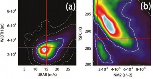
Figure 2. Probability maps for average wind speed (UBAR) and mountain width (WIDTH) (a); atmospheric stability (NM2) and surface temperature (TSFC) (b). Red lines show control values, bright areas those of highest probability.
Figure 2a shows an example of a 2D probability map for UBAR, the mean wind speed flowing toward the mountain, and WIDTH, the half-width of the mountain itself. Red lines indicate the control values of wind speed and half-width. The bright white-blue area indicates that the values of wind speed and half-width within that area have the highest probability of producing precipitation in a pattern identical to the control case. The single, well-defined mode of high probability implies that the cloud model is sensitive to these parameters.
The results agree with the current understanding of wind speed and mountain half-width in the orographic precipitation system: as mountain width increases, stronger winds are needed to produce the same amount of lift and precipitation. If the mountain is too small or the wind too weak, there will not be enough lift to produce precipitation similar to the control case. Some other parameter combinations don’t show such a clear-cut relationship.
For example, the probability map of surface temperature and atmospheric stability (Figure 2b) has multiple probability bull’s-eyes, suggesting a complex, non-unique solution. This was hinted at in Figure 1, where a 2-K temperature difference had a large impact on mountain precipitation. As atmospheric stability increases, the surface temperature must decrease in order to reach saturation and produce precipitation. The two solutions shown in the probability map describe two different atmospheric states—one cool and less stable, one warm and more stable—that produce similar precipitation.
Use of statistical methods in orographic precipitation research has opened the door for more and better experimentation with numerical models. The MCMC algorithm allows us a revolutionary look into the orographic precipitation system, and makes model output available for a host of different combinations of parameters. Probability maps, plots of the precipitation response to parameter changes, and other useful interpretations reveal much about the system’s sensitivity and relationships between parameters and precipitation output.
In this current economic climate—with grant cuts and decreased lab time, Bayesian statistics can help us solve problems in the actual climate. The tools generated through Bayes theorem help us to better comprehend mountain precipitation and its relationship to the environment, and improve forecasting of the rain and snow that affect mountainous regions.
Welcome to the newly regenerated Down to Earth department! Previous Down to Earth correspondent, Rachel Berkowitz, has taken the next step in her career. The department will be taking a different direction inspired by research presented by students at the annual meeting of the American Meteorological Society. Down to Earth will now feature the research of atmospheric science graduate students from around the country. The monthly articles will describe graduate research that ranges from theory to application, from the Earth’s surface to orbiting satellites, and from the molecular to the planetary scale. This inaugural article is written by the department’s editor, Samantha Tushaus from the University of Michigan Department of Atmospheric, Oceanic, and Space Sciences.
For the UNESCO section chief, “striking a balance between global coherence and respect for national ownership and cultural diversity is both essential and complex.”