Satellite altimetry quantifies the alarming thinning of Arctic sea ice
DOI: 10.1063/1.3226704
The Arctic Ocean’s floating sea-ice cover waxes and wanes with the seasons. The icecap grows in the fall when the hours of sunlight shorten and intense cold sets in. When long summer days return, ice floes melt or are driven by wind and ocean currents into the North Atlantic Ocean. A quarter century ago, the coverage ranged from about 7 million to 16 million km2 between late summer and the following March.
Since 1978, when satellites began routinely monitoring the Arctic, the extent covered by perennial ice—that which survives the summer melt—has declined by close to 10% per decade, at least until 2007. In September of that year, the summer ice extent plummeted to a record low 4.2 million km2, down 23% from a previous record low in 2005. The perennial ice lost in those two years alone covered an area almost twice the size of Texas. (For a broader perspective on changes in the Arctic, see reference and the article by Josefino Comiso and Claire Parkinson in Physics Today, August 2004, page 38 .)
The trend, no doubt, reflects the Arctic’s response to the warming of Earth’s climate. And the recent acceleration is worrying. The Arctic is particularly sensitive thanks to the ice albedo–ocean feedback at work there. For example, a drop in ice cover increases the absorption of solar radiation in the ocean, warms the water, prolongs the melting, and reduces the ice cover yet further. As figure 1 shows, the impact of those changes on the Arctic’s human inhabitants can be severe.

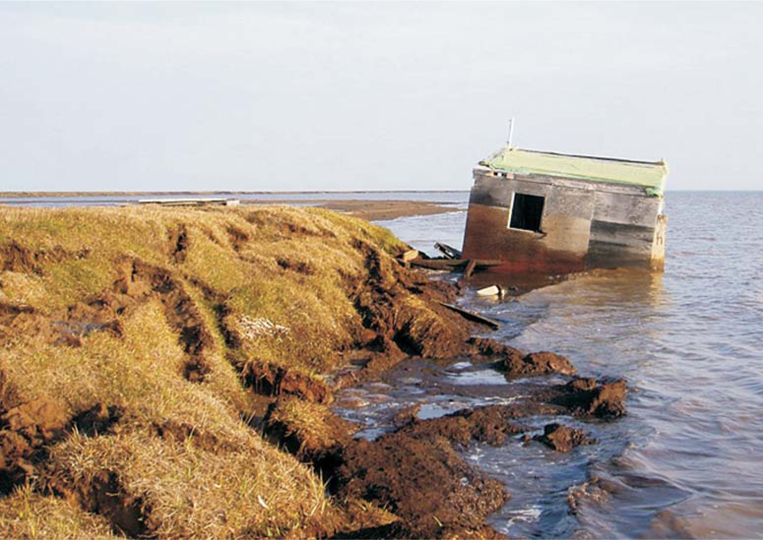
Figure 1. A cabin along the Alaskan coastline has collapsed into the Beaufort Sea because of coastal erosion. Warming sea temperatures, rising sea levels, exposure to choppy waves, and the thawing of ice-rich bluffs have contributed to an increase in the erosion rate—from 8.7 m/year between 1979 and 2002 up to about 14 m/year between 2002 and 2007—along a stretch of that coastline.
(Photo courtesy of Benjamin Jones, US Geological Survey.)
For a richer, more quantitative picture of how the icecap responds to climate, more than areal details are needed: Ice thickness controls the exchange of heat between ocean and atmosphere. Since the 1950s, submarine-mounted upward-looking sonar has provided data on ice draft, the submerged portion (roughly 89%) of the ice sheet. But those data are largely anecdotal, limited to one-dimensional transections under certain regions of Arctic ice; some of the data even remains classified. What’s more, the speed of the ice floes, which can reach 40 km/day, makes it tricky to keep track of the dynamic Arctic.
The sparse measurements kept researchers heavily reliant on numerical models. But those models have their own limitations: Simulations alone cannot entirely clarify whether the decline in ice extent and thickness is controlled mainly by thermodynamics—melting and freezing from radiative or thermal flux—or by mechanical forcing, such as changes in ice circulation from wind and ocean stress.
For basinwide estimates of ice thickness, researchers had to wait until 2003, when Seymour Laxon and colleagues from University College London published the first radar-altimetry data taken from the European Space Agency’s ERS-1 and ERS-2 satellites. 2 In January of that year, NASA launched its own satellite, ICESat, also designed to measure the thickness of polar ice sheets. But aboard ICESat is a lidar system whose 70-m laser footprint is an order of magnitude finer than the earlier radar and which operates at an orbital inclination a few degrees higher than that of the ERS satellites. The higher inclination allows it to read reflections from an additional 2 million km2.
Ronald Kwok (NASA’s Jet Propulsion Laboratory) and colleagues from NASA and the University of Washington have now published what may be the most accurate and comprehensive set of maps yet of the entire Arctic basin, based on 10 lidar surveys taken between 2003 and 2008. 3 “The timing is perfect,” comments Hajo Eicken (University of Alaska Fairbanks), “because it captures a period in which the ice extent went through a three-decade minimum—what many of us expect is a record minimum for the past century or longer. Armed with details about the jumps and spurts in the ice pack’s volume, mass, and heat capacity, theorists can fine-tune their models.”
Archimedes’ principle
ICESat’s lidar system only senses radiation scattered from surfaces. Fortunately, it can distinguish to within 2 cm height differences between the sea surface and nearby ice floes. After measuring that “freeboard” portion, assuming hydrostatic equilibrium, and knowing the densities of ice, snow, and seawater, Kwok and company could calculate the rest—how much ice must lie underwater. Accounting for the snow and its drift atop the ice was more challenging. Team members used precipitation rates calculated from meteorological models and found they could estimate the likely snow cover well enough to derive ice-thickness estimates that were consistent with those from submarines and fixed mooring sites below the surface.
Another complication is the heterogeneity of sea ice in the Arctic. As sea ice ages, brine drains out of it. Older, multiyear (MY) ice, that which has survived one or more melt seasons, is much fresher than seasonal, first-year (FY) ice. The loss of salinity—in effect, the filling of brine drainage channels with air bubbles—also makes old ice more reflective than seasonal ice—at least a third more reflective to solar radiation, according to Eicken.
That difference makes the ice classes distinguishable by microwave scattering experiments. To resolve their thickness data into FY and MY components, Kwok and company processed their ICESat data in tandem with scatterometry from another satellite known as QuikSCAT.
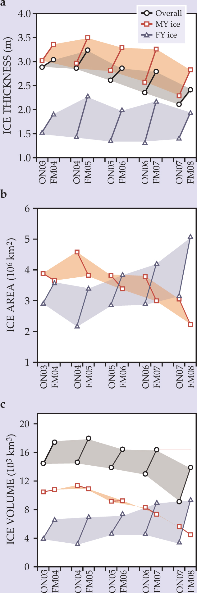
The results, outlined in figure 2, explain why the ice pack has become so vulnerable to climatic variations. In general, older ice is thicker than younger ice and serves as an insulating buffer at the end of a melt season. The years surveyed by ICESat, though, have seen the ice sheet thin by close to 0.7 m on average, nearly all of it from the MY component. Indeed, between 2004 and 2008, the winter cover of MY ice shrank 42%, or 1.5 million km2. During the same period, the volumetric MY-ice contribution thinned by 57%—so much that FY ice became the dominant type in 2008 for the first time on record. On average, MY ice is thickest (5-6 m) next to Ellesmere Island and the Greenland coast and progressively thins out toward the central Arctic and the coast of Siberia.

Figure 2. Sea ice can be parsed by age into first-year (FY) and multiyear (MY) components. The thicker MY ice supports a large thermal gradient between warm ocean and cold atmosphere. (a) Over the five-year span of ICESat’s 10 surveys of the Arctic basin, the fall sea ice thinned, on average, from 2.9 m to 2.2 m. Each year’s melt exceeded growth, which took a toll on the MY-ice reserve. The fall FY thickness component remained close to 1.4 m each year. (Overall values are weighted by the area occupied by MY and FY components; ON and FM refer to October/November and February/March.) (b) The seasonal cycles for FY and MY components of area covered are opposite because of the relative ease of FY-ice growth and export of ice floes into the Atlantic Ocean. (c) Between 2003 and 2008 a near reversal occurred in the contributions of FY and MY ices to the total volume. At the start of the survey, 62% was stored as MY ice; by 2008 the MY component had dropped to 32% of the total.
(Adapted from ref. 3.)
Consequences
Thinner ice at the start of a melt season leads to more open water at the end of it. The extra energy stored in the ocean during summer months is then given back to the atmosphere as heat in the fall. According to the National Oceanic and Atmospheric Administration’s James Overland, air temperatures over those ice-free areas can be 5–6 °C warmer than over covered areas. Rising of the warm air into the troposphere can then “tilt” regional atmospheric pressure surfaces and modify wind patterns. Indeed, persistent southerly winds that formed in the summer of 2007 between high pressure over the Beaufort Sea north of Alaska and low pressure over eastern Siberia are thought to be responsible for the circulation of warm winds that led to excessive melt and the export of ice from the Siberian coast that year.
The influence of recent warm years and wind-driven sea ice, Overland argues, has thinned Arctic ice to the point that natural climate variability may kick the ice albedo feedback process into high gear. Based on models that couple ice, ocean, and atmosphere, he projects the loss of most summer ice within the next 30 years. 4 “Reversing recent trends would take several cold years in a row, which is probably not in the cards. We’re on a one-way trip.”
The Arctic is already transforming: Last summer was the second in a row in which the Northwest Passage was navigable through the Canadian archipelago; fisheries from northern Norway to the Bering Sea are expanding farther north; animals are losing their habitats; and the retreat of ice from coastlines is exacerbating erosion (see figure 1).
Perhaps most intriguing, and uncertain, is the role that ocean waters play in the melting of Arctic ice. Dense with salt and carrying enough heat to melt the entire cap, the Atlantic Ocean enters the Arctic some 250 m below the surface, separated only by a layer of colder, less saline water.
References
1. M. C. Serreze, M. M. Holland, J. Stroeve, Science 315, 1533 (2007); https://doi.org/10.1126/science.1139426
J. Stroeve et al., Eos Trans. Am. Geophys. Union 89, 13 (2008). https://doi.org/10.1029/2008EO0200012. S. Laxon, N. Peacock, D. Smith, Nature 425, 947 (2003). https://doi.org/10.1038/nature02050
3. R. Kwok et al., J. Geophys. Res. 114, C07005 (2009). https://doi.org/10.1029/2009JC005312
4. M. Wang J. E. Overland, Geophys. Res. Lett. 36, L07502 (2009). https://doi.org/10.1029/2009GL037820
5. B. M. Jones et al., Geophys. Res. Lett. 36, L03503 (2009). https://doi.org/10.1029/2008GL036205


