Nobel Prize in Physics Honors Theoretical Work on Superconductivity and Superfluidity

The Royal Swedish Academy of Sciences has selected Alexei A. Abrikosov of Argonne National Laboratory, Vitaly L. Ginzburg of the P. N. Lebedev Physical Institute in Moscow, and Anthony J. Leggett of the University of Illinois, Urbana-Champaign to receive the 2003 Nobel Prize in Physics. The trio is being recognized for their “pioneering contributions to the theory of superconductors and superfluids.” It is not the first Nobel prize to honor such theoretical work. Medals have previously gone to Lev Landau, who contributed to the understanding of ⁴He superfluidity, and to John Bardeen, Leon Cooper, and Robert Schrieffer, who together offered a microscopic theory of low-temperature superconductivity (the BCS theory).

The current Nobel Prize recognizes other key contributions to this body of work. In 1950, seven years before the BCS theory appeared, Ginzburg, together with Landau, formulated a phenomenological, or macroscopic, treatment of the superconducting state. That treatment remains a useful approach even for the high-temperature superconductors, whose microscopic properties are not yet fully understood. In the mid-1950s, Abrikosov used the Ginzburg–Landau (GL) equations to develop a theory of type II superconductors and originated the idea that magnetic fields can penetrate in vortex-like flux lines. In 1972, Leggett showed how pairing in ³He could be used to explain puzzling observations and predict new phenomena in the superfluid’s nuclear magnetic resonance (NMR) behavior. Pierre Hohenberg of Yale University notes that the prize also serves, in a way, as a posthumous second Nobel for Landau.

A phenomenological approach

Landau headed a renowned school of theoretical physics at the Institute for Physical Problems when Ginzburg joined the nearby Lebedev Institute in the 1940s as a young theorist. (See the reminiscences of Landau by I. M. Khalatnikov and by Ginzburg in Physics Today, May 1989, pages 34 and 54 , respectively.) Influenced by Landau’s work on superfluidity, Ginzburg began applying some of Landau’s ideas to describe superconducting phenomena. In 1950, the two collaborated on formulating a now classic approach.

Others by then had contributed useful ideas. In 1934, Cornelis Gorter and Hendrik Casimir had introduced a two-fluid model, the fluids being normal electrons and constituents of a superconducting state. The next year, the brothers Fritz and Heinz London formulated a macroscopic description of a superconductor, particularly its electromagnetic properties. The London approach, however, could not treat the behavior of magnetic fields in thin superconducting films. Nor could it properly describe the boundary between a normal and a superconducting region.

Ginzburg and Landau’s formulation overcame those limitations. ^1,2 Their work followed Landau’s earlier approach to second-order phase transitions. To characterize the change of a system from a disordered to an ordered state, Landau had introduced the concept of an “order parameter.” The value of the order parameter grows as one passes through the critical temperature from zero (characterizing a disordered state) to nonzero (for an ordered, or aligned, state). For a ferromagnetic transition, Landau showed that the spontaneous magnetization functions as an order parameter.

In the case of the normal-to-superconducting transition, Ginzburg and Landau chose an order parameter ψ to represent what they called “the effective wavefunction of the superconducting electrons.” The order parameter ψ was a complex number, and its square was what we now know as the density of superconducting pairs.

After writing the free energy in terms of the order parameter, adding terms corresponding to the kinetic energy and the magnetic energy, and minimizing the free energy, the theorists came up with the well-known Ginzburg–Landau equations:

$$\begin{array}{c}\left(1/2m^{*}\right){\left(-iħ\nabla -e^{*}A/c\right)}^2\psi +\alpha \psi +\beta {\left|\psi \right|}^2\psi =0\\ j=\nabla \times H=e^{*}ħ/\left(2m^{*}i\right)\left({\psi }^{*}\nabla \psi -\psi \nabla {\psi }^{*}\right)+e^{*2}/\left(m^{*}c\right){\left|\psi \right|}^{2}A,\end{array}$$

where m*, e*, and β are constants; α is a function of temperature; H is the external magnetic field; and A is the vector potential. The second of the two equations has the same form as the usual expression for the current density in quantum mechanics. The first resembles the Schrödinger equation for an electron in a magnetic field, with the exception of the term that’s nonlinear in ψ.

The GL equations successfully explained the existing experimental observations, including the critical magnetic field in thin films—the field value at which the external field is expelled from the film’s interior. Once the BCS theory appeared, Lev Gor’kov (now at the National High Magnetic Field Laboratory in Gainesville, Florida) used the new theory to derive the GL equations near the critical temperature. ³ Gor’kov made a big contribution, says William Brinkman of Princeton University, not only by showing the equivalence of the macroscopic and microscopic approaches, but also by introducing a method that has wider applicability than the BCS equations.

Type II superconductors

Despite its many successes, the GL equations failed to explain some experiments on superconducting thin films done in the early 1950s by N. V. Zavaritskii. At the time, both Zavaritskii and Abrikosov were Moscow State University students. Zavaritskii had grown some thin films that had a rather amorphous structure. In those films, the critical magnetic field did not follow the predictions of the GL equations.

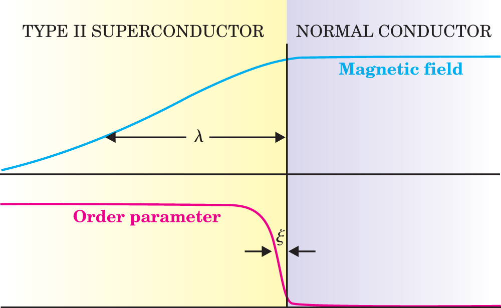
Abrikosov and Zavaritskii realized that the problem might lie in the value assumed for the parameter κ, which arises in some solutions to the GL equations. The parameter κ is the ratio of the London penetration depth λ to the coherence length ξ. The two lengths are the characteristic distances for the exponential decay of the magnetic field and superconducting order parameter, respectively, near a boundary between normal and superconducting regions. For most superconductors known in the 1950s, κ was much smaller than 1. Abrikosov and Zavaritskii speculated, however, that for the amorphous films, κ might be much larger than 1.

If one puts $\kappa >1/\sqrt{2}$ in the GL equations, the surface energy at the boundary between superconducting and normal regions will be negative. A negative surface energy means that it’s favorable to form such boundaries, as explained in figure 1. Ginzburg and Landau had only considered the common case in which $\kappa <1/\sqrt{2}$ and the surface energy is positive. In the negative-energy case, normal regions can nucleate within a superconductor.

Using the GL equations, Abrikosov calculated the critical fields for thin films with $\kappa >1/\sqrt{2}$ and found good agreement with Zavaritskii’s data. In the 1952 paper reporting his findings, ⁴ Abrikosov called such materials “superconductors of the second type,” known now as type II. But Abrikosov was not widely credited for that finding at the time, because his paper was never translated into English.

Today we know bulk type II superconductors as ones with two critical fields: an upper critical field, H _c2, at which the material becomes superconducting even though the external field still penetrates the material, and a lower critical field H _c1 at which the superconductor completely expels the field. In 1937, Lev V. Shubnikov and his group at the Ukrainian Physico-Technical Institute in Kharkov, following earlier work, had measured those two critical fields in alloys. Observers at the time explained away the results as being caused by inclusions of normal metal regions in the samples.

The mixed state

After the work on thin films, Abrikosov studied bulk superconductors having $\kappa >1/\sqrt{2}$ . He found that below H_c2 there were points in his solution where the wavefunction ψ went to zero. In a closed line integral around such a point, the phase angle of ψ must change by a multiple of 2π. Ginzburg and Landau had put into their equations a complex order parameter, with a phase angle, but Abrikosov was the first to make explicit use of that angle.

“I concluded,” Abrikosov recalls, “that below a limiting critical field, a new and very peculiar thermodynamic phase arose, with a periodic distribution of order parameter, magnetic field, and current, which I called the mixed state.” Specifically, Abrikosov came up with the idea of vortices: Filaments of normal region are arranged periodically within the superconductor; magnetic flux lines thread through those filaments and supercurrents flow around the flux lines. Each point at which ψ = 0 corresponds to the core of such a vortex.

Abrikosov calculated that the vortices would form a triangular lattice near H _c1 and a square lattice near H _c2. The triangular lattice turned out to be favored at both fields. Abrikosov says that many experimentalists firmly believed in the vortex lattice only after they saw the first images of triangular flux lattices, produced in 1967.

When Abrikosov heard, in 1955, about Richard Feynman’s proposal of vortices in superfluid ⁴He, he gained confidence in his own ideas about vortices. He worked out the theory and published it in 1957. ⁵

Abrikosov did his calculations based on the GL theory, which is valid for temperatures near T _c. Many other theorists, including Gor’kov, pitched in, using the BCS approach to extend the theory of type II superconductors to lower temperatures.

Superfluidity in ³He

Once researchers knew that electrons could pair in a superconductor, they began thinking about how fermions might pair in other condensed matter systems. In the late 1950s, long before David Lee, Douglas Osheroff, and Robert Richardson found ³He superfluidity at Cornell in 1972 (see Physics Today, page 17, December, 1996 ), theorists speculated that ³He atoms (fermions) might pair up to form bosons and, perhaps, a superfluid.

In the mid-1960s, Leggett was a postdoc at Illinois, where experimentalist John Wheatley had shown that, below 100 mK, ³He could be well described by Landau’s Fermi liquid theory. Leggett corrected Landau’s theory for the effect of BCS pairing and successfully predicted some superfluid properties. ⁶ Philip Anderson of Princeton says that this work was Leggett’s best: “He predicted the temperature dependence of the susceptibility in the B phase with remarkable accuracy, seven years ahead [of its measurement.]”

Atoms of ³He are not apt to pair in a state with zero angular momentum (the isotropic s-wave state) because the repulsion of the two atoms pushes them too far apart. A number of theorists thus suggested that ³He atoms might pair either in a p-wave (with angular momentum l = 1) or a d-wave (l = 2) state. Those states are anisotropic, which means that the superfluid can have different properties in different directions.

Today we know that ³He atoms pair in a p-wave state. Consequently, the total wavefunction is antisymmetric under an exchange of spatial coordinates. For the overall wavefunction to be antisymmetric (as the Pauli principle demands), the wavefunction must be symmetric under an exchange of spin coordinates of the two particles. The allowed configurations for pairs of spin are (↑↑), (↓ ↓), and $\left(\uparrow \downarrow +\downarrow \uparrow \right)/\sqrt{2},$ , and the total spin is S = 1.

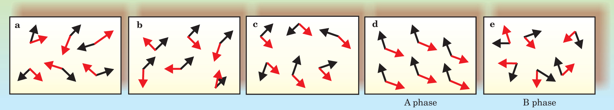
To represent a ³He superfluid by an order parameter in a GL-type treatment is far more complicated than in the case of a ferromagnet, in which a single number stands for the spontaneous magnetization. ³He can have three kinds of symmetry breaking: the rotational symmetry in spin space, the orbital rotational symmetry, and the gauge symmetry associated with the pair condensate. Some possible broken-symmetry states are shown in figure 2. As Leggett was to show in the 1970s, describing all possible states requires a tensor order parameter with nine complex components rather than the simple scalar that depicted symmetry breaking in a uniaxial ferromagnet. That’s what makes the anisotropic superfluid at once intriguing and challenging.

In the early 1960s, Anderson and Pierre Morel calculated the properties of superfluid pairs both in a d-wave state and in a p-wave state. ⁷ The p-wave state they considered—the so-called ABM state for Anderson, Morel, and, later, Brinkman—contained only the (↑ ↑) and (↓ ↓) spin configurations. In 1963, Roger Balian and N. Richard Werthamer found that by including the $\left(\uparrow \downarrow +\downarrow \uparrow \right)/\sqrt{2}$ state they would get a lower energy p-wave state (the BW state). ⁸ Yuri A. Vdovin did similar work in the Soviet Union.

When Lee, Osheroff, and Richardson discovered superfluid ³He in 1972, they saw two phases, each one in a different region of temperature and pressure. Anderson and Brinkman, working at Bell Labs, soon showed that the experimentally observed “A” and “B” phases corresponded, respectively, to the ABM and BW states. A third phase, “A₁,” has only the (↑ ↑) state.

Nuclear magnetic resonance

Although most researchers immediately interpreted the 1972 Cornell experiment as proof of the predicted superfluid ³He, Leggett says he was not convinced, largely because of two puzzles presented by the data: One was the existence of two phases (later three). Leggett didn’t understand how different phases could be stable in different regions of pressure and temperature. The calculations by Anderson and Brinkman answered the question by showing that the interaction between atoms is modified by the formation of Cooper pairs. This feedback made the energy of each state dependent on temperature and pressure.

A second puzzle was the behavior of the NMR signal. Leggett himself tackled that puzzle. Experimenters were measuring unexpectedly large shifts in the resonant frequency for the A phase and no shift in the B phase. The NMR shifts reflect the nuclear dipole–dipole interaction, which, for ³He, should be tiny. Leggett recognized, though, that all the magnetic moments might align and add coherently in the superfluid phase so that the individual signals were multiplied by something like Avogadro’s number, 10²⁴.

Soon after receiving the NMR measurements from the Cornell group in 1972, Leggett did a sum rule calculation and predicted that the frequency shift should be on the order of megahertz. At first, he was discouraged because he had mistakenly thought the experimental value was on the order of kilohertz, but soon learned that the experimental shifts were fully as large as he predicted.

Leggett next formulated a general theory aimed at understanding how one might get shifts in the NMR frequency. ⁹ To get such shifts requires the breaking of spin–orbit symmetry, he says. According to Anderson, Leggett’s paper “shows just exactly how to do the spin dynamics and exactly how to describe the internal order parameter.” David Mermin of Cornell stresses that the system is a highly technical, nonintuitive one involving a tensor order parameter. “Tony’s theory of a spin dynamics for the order parameter was a highly creative vision,” he says.

Leggett’s theory explained the large frequency shift in the A phase and the absence of a shift in the B phase. Furthermore, Leggett made predictions of the shifts one might see if the magnetic field were parallel, rather than perpendicular, to the surface. Osheroff found that these longitudinal resonances were exactly as Leggett had predicted.

Biographies

Born in Moscow in 1928, Abrikosov earned his PhD in physics in 1951 and a doctorate in physical and mathematical sciences in 1955 at the Institute for Physical Problems. From 1965 to 1988, he headed the condensed matter theory division of the Landau Institute for Theoretical Physics. He was director of the Institite for High Pressure Physics in Troitsk, near Moscow, from 1988 to 1991. In 1991, Abrikosov went to Argonne, where he is now a Distinguished Argonne Scientist.

Ginzburg, now 87, was born in Moscow. He received a PhD in physics at the University of Moscow in 1942. He has been associated with the Lebedev Institute since 1940, and directed the theory group there from 1971 to 1988.

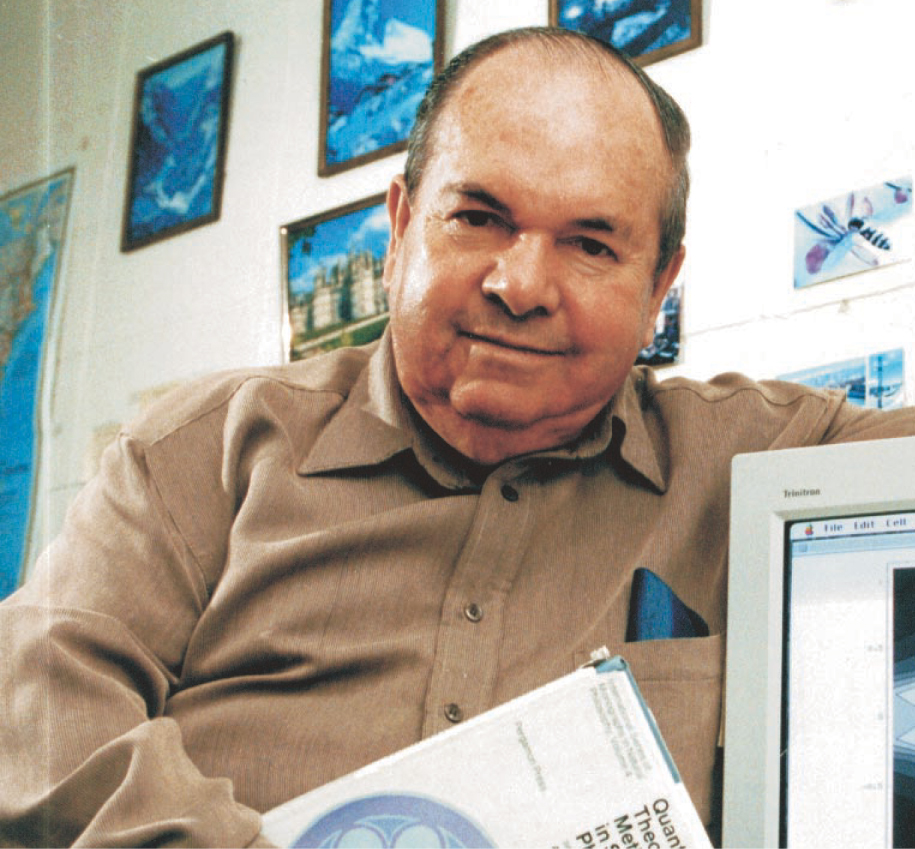
Leggett, born in London in 1938, earned his doctorate in physics from Oxford University in 1964. After doing postdoctoral work at Illinois and at Oxford, he joined the faculty of the University of Sussex in 1967. He left Sussex in 1983 to assume his current position as the John D. and Catherine T. MacArthur Professor of Physics at Illinois.

References

1. V. L. Ginzburg, L. D. Landau, Zh. Eksp. Teor. Fiz. 20, 1064 (1950).
2. See Ginzburg’s account in V. L. Ginzburg, Phys. Usp. 40, 407 (1997) https://doi.org/10.1070/PU1997v040n04ABEH000230 .
3. L. P. Gor’kov, Sov. Phys. JETP 36, 1364 (1959).
Sov. Phys. JETP 37, 998 (1960).4. A. A. Abrikosov, Dokl. Akad. Nauk SSSR 86, 489 (1952).
5. A. A. Abrikosov, Sov. Phys. JETP 5, 1174 (1957).
6. A. J. Leggett, Phys. Rev. 140A, 1869 (1965) https://doi.org/10.1103/PhysRev.140.A1869 .
7. P. W. Anderson, P. Morel, Phys. Rev. 123, 1911 (1961) https://doi.org/10.1103/PhysRev.123.1911 .
8. R. Balian, N. R. Werthamer, Phys. Rev. 131, 1553 (1963) https://doi.org/10.1103/PhysRev.131.1553 .
9. A. J. Leggett, Phys. Rev. Lett. 31, 352 (1973) https://doi.org/10.1103/PhysRevLett.31.352 .