Gyromagnetic ratio of a lone trapped electron is measured to better than a part per trillion

A new paper in Physical Review Letters brings word of the first improvement in two decades in the measurement of the electron’s gyromagnetic ratio. ¹ The new measurement by Gerald Gabrielse’s group at Harvard University of g _e, the electron’s magnetic moment in units of the Bohr magneton (eħ/2m _e), carries an estimated uncertainty of 7.6 parts in 10¹³. That’s a sixfold improvement on the celebrated precision of the 1987 measurement that won a Nobel Prize for University of Washington experimenter Hans Dehmelt.

Quantum electrodynamics predicts the value of g _e in terms of the fine-structure constant α = 1/137.03. … Those two fundamental dimensionless constants characterize the electron’s interaction with the electromagnetic field. The new g _e measurement, together with a recent numerical calculation of high-order QED Feynman diagrams contributing to g _e, yields a determination of α ten times more accurate than any competing method has been able to provide.

The new α determination subjects QED, already the most precisely verified theory in all the natural sciences, to its most stringent test yet. That test and the limits it puts on possible new physics beyond QED and the standard model of particle interactions are discussed in a companion paper ² coauthored by the Harvard experimenters and theorists Toichiro Kinoshita (Cornell University) and Makiko Nio (RIKEN). Kinoshita and Nio carried out the computer calculation of the 891 eight-vertex QED Feynman diagrams needed to predict g _e to the new measurement accuracy. ³

Anomalous magnetic moment

If the electron were simply a spinning ball whose charge distribution faithfully followed its mass distribution, g _e would be 1. Indeed g is 1 for the contribution of an electron’s orbital motion (in an atom or a magnetic field) to its magnetic moment. Paul Dirac’s relativistic wave equation of 1928 not only required the electron to have an intrinsic spin of ħ/2; it also predicted that g _e should be exactly 2. But with the formulation of QED in the late 1940s, Julian Schwinger pointed out the first of an infinite series of small corrections to Dirac’s g _e required by the new theory. Successive terms, describing ever more couplings of virtual photons, involve successively higher powers of α/π.

The so-called anomalous magnetic moment a _e due to QED and any other small corrections to the Dirac g _e is defined by

$$a_{\text{e}}\equiv \left(g_{\text{e}}-2\right)/2.$$

To the first power in α/π, as calculated by Schwinger, a _e = α/2π. That’s roughly a 0.1% correction. Since the 1940s, theory and experiment have been confronting each other with ever-finer predictions and measurements of the electron’s anomalous magnetic moment.

By the time g _e is measured to a part in 10¹¹, comparison with theory requires that one take account of predictions beyond QED, involving first the electromagnetic interactions of the electron’s heavier siblings (the µ and τ leptons) and then the strong and weak interactions of quarks and leptons. Any unreconciled anomalous moment remaining after all that would be regarded as evidence of new physics beyond the standard model.

The trap

Precision measurements of g _e exploit the near equality of the frequencies of two periodic motions of the electron in a magnetic field. In a uniform field B, the electron executes cyclotron orbits of frequency v _c = eB/2πm _e in the plane normal to B. In the same magnetic field, the precession frequency v _s of the electron’s intrinsic spin is v _c g _e/2, so that a _e equals the small fractional difference (v _s – v _c)/v _c.

To measure g _e, Gabrielse and company confined single electrons for months at a time in a small Penning trap (see figure 1) whose design has evolved from the one Dehmelt and company used in the 1980s. An innovation of the new trap is its carefully designed cylindrical symmetry, which contributes significantly to precision by making it possible to understand and exploit distortions due to the confinement of radiation in the small enclosure. Those so-called cavity-QED effects bedeviled measurements in earlier Penning traps.

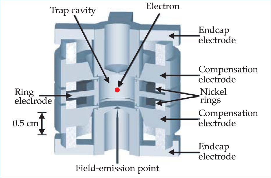
The trap’s electrodes create a quadrupole electric potential whose vertical restoring force confines the electron near the center and makes it oscillate harmonically along the vertical (z) axis with a frequency v _z near 200 MHz. Horizontal confinement in cyclotron orbits is provided by an approximately uniform vertical magnetic field of about 5 tesla that yields v _c near 150 GHz in the microwave regime.

Because the trap is maintained at a temperature of 100 mK, thermal radiation is too feeble to excite the electron’s cyclotron motion out of its lowest quantum level. “Ours is the first determination of g _e from observed transitions between the lowest quantum states of a single trapped electron,” says Gabrielse. “With quantum-nondemolition measurements, we fully resolve the lowest cyclotron and spin levels, while disturbing them as little as quantum mechanics allows.”

Aside from small corrections, the energy of a one-electron eigenstate of cyclotron motion and spin orientation in the trap is

$$E\left(n,m_s\right)=\left(n+1/2+m_s{g}_e/2\right)h{v}_c,$$

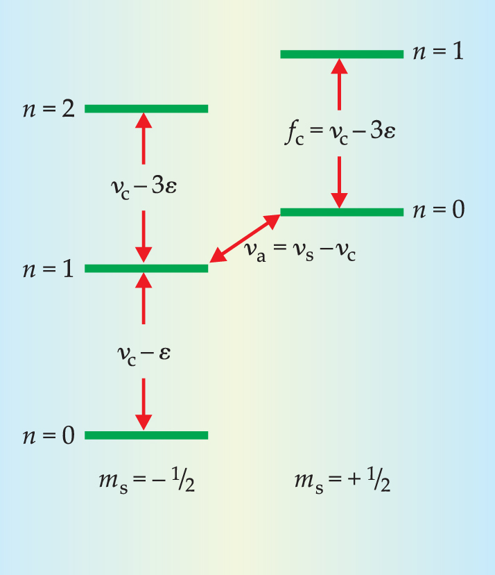
where n = 0, 1, 2, … is the cyclotron-orbit quantum number and m _s = ±1/2 gives the orientation of the electron’s intrinsic spin with respect to the upward-pointing B. For their determination of g _e, Gabrielse and company used what they call quantum-jump spectroscopy to measure, within a few parts per billion, two excitation frequencies (see figure 2): the applied microwave frequency (essentially v _c) needed to induce a cyclotron-level jump, and the RF frequency v _a = v _s – v _c that induces an “anomaly” spin-flip transition between the almost coincident (n, m _s) levels (0, +1/2) and (1, −1/2).

Detecting transitions

To measure the precise excitation frequencies, the Harvard group had to know the electron’s quantum state before and after each attempted excitation. That’s where the harmonic axial oscillation comes in. The axial frequency v _z depends primarily on the strength of the electric quadrupole restoring force. But ferromagnetic nickel rings slightly distort the trap’s otherwise uniform magnetic field into a small “magnetic bottle” at the center. The bottle’s weak field gradients couple to the magnetic moments generated by the electron’s intrinsic spin and its cyclotron orbit.

The resulting effect on the trap’s vertical restoring force is a few-parts-per-10⁸ dependence of v _z on n and m _s. Figures 3(a) and 3(b) show the impressive clarity of the effect, made manifest by an innovative self-excited oscillator (SEO) that amplifies the tiny RF signal induced by the axial motion and feeds it back to the electron to enhance and stabilize its axial oscillation.

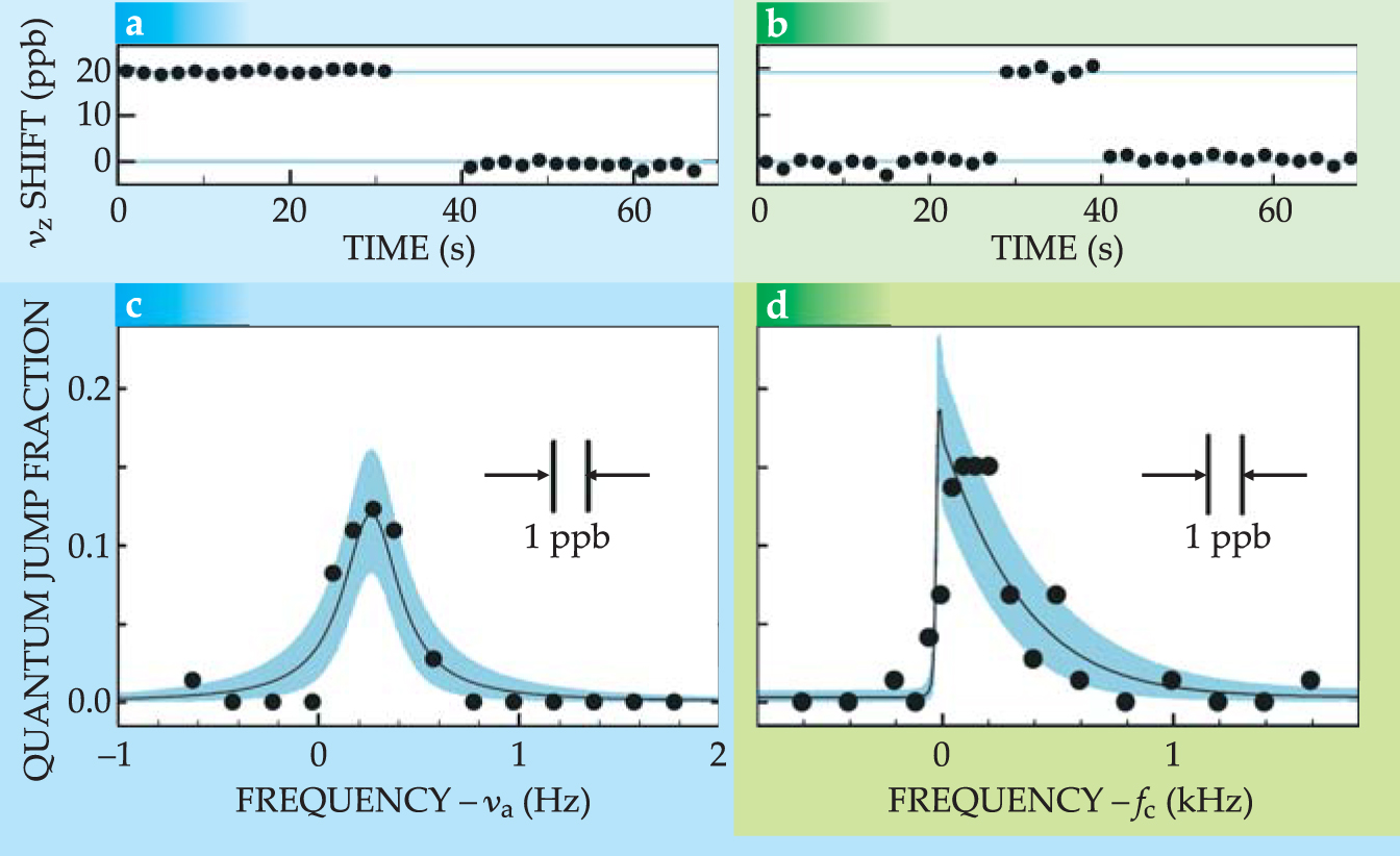
The downward v _z step in 3a signals the spontaneous decay of the cyclotron orbit to the spin-down ground state made possible by an induced spin flip out of the spin-up ground state. The up and down steps in 3b record an induced excitation out of the spin-up ground state without a spin flip, followed about 10 seconds later by spontaneous decay back to that ground state.

Ordinarily an excited cyclotron state would decay spontaneously in a fraction of a second. The state’s greatly extended lifetime in Gabrielse’s cylindrical trap, which makes it much easier to know that a cyclotron excitation has occurred, results from cavity-QED suppression of microwave radiation modes. The trap also has another, less obviously useful cavity-QED effect. It can actually shift g _e from its true value in an unbounded vacuum. In fact, the new Harvard experiment demonstrates such a cavity-QED shift for the first time. But the trap’s geometry allowed Gabrielse and company to show that the shift becomes significant only when the cyclotron frequency approaches particular resonant modes of the cavity. Therefore, by tuning B to put v _c between offending modes that would tug it in opposite derections, they were able to convince themselves that any cavity shift of g _e was negligible.

Quantum-jump spectroscopy

A microwave coupler (not shown in figure 1) can inject a pulse of radiation into the Penning trap at any microwave frequency the experimenters choose. Similarly, they can inject RF radiation by imposing an RF pulse on the endcap electrodes. The Harvard group began each of its many experimental runs by examining v _z with the SEO to see that the electron was in the spin-up ground state, or nudging it there if necessary. Then the experimenters would apply one of a frequency-stepped sequence of RF pulses (figure 3(c)) or microwave pulses (figure 3(d)).

After each pulse, they interrogated the SEO again to see if the pulse had initiated a quantum jump. The figure of merit in this kind of spectroscopy, plotted against pulse frequency in figures 3(c) and 3(d), is the fraction of pulses that succeed in initiating the intended quantum jump. A sudden rise in that fraction with increasing frequency indicates the sought-after excitation frequency.

In figure 3(c), stepping the frequency of imposed RF pulse reveals the anomaly excitation frequency v _a = v _s – v _c. And in 3d, stepping the microwave-pulse frequency reveals the relevant cyclotron-excitation frequency f _c ≡ v _c – 3ε. The ε term is a small but not negligible relativistic correction. Note that such relativistic corrections spoil the usual textbook simplification that all single-step cyclotron excitations have the same spacing (see figure 2).

The Harvard group carried out such runs again and again with the same electron sitting in the same painstakingly stabilized magnetic field—usually late at night when electrical and mechanical perturbations were minimal. From all those runs and a model of the spectroscopic line shapes, the group determined v _a and f _c with the requisite precision to yield the anomalous moment a _e to 7 parts in 10¹⁰. That’s much better than one could know the trap’s magnetic field—or, for that matter, the electron’s mass. But, happily, those dimensional quantities cancel out when one measures the fractional difference between the frequencies that induce spin flip and cyclotron excitation.

QED survives its toughest test

Kinoshita and Nio have recently completed ³ the impressive task of numerically computing the 891 eight-vertex Feynman diagrams that contribute to the (α/π) ⁴ term of the QED prediction of g _e. Together with the new experimental result, that calculation (plus small additions for standard-model physics beyond QED) yields a new determination of α with an uncertainty of only 7 parts in 10¹⁰.

That’s an order of magnitude better than any measurement of α that does not involve g _e. The best determination of α by means independent of g _e come from recently reported measurements with rubidium and cesium atoms. ⁴ They yield α to about 7 parts in 10⁹. Even though the Kinoshita–Gabrielse α has a 10 times smaller uncertainty, its excellent agreement with the Rb and Cs results is in fact the best test to date of QED.

So there’s still no sign of a discrepancy that might point the way to new physics beyond the standard model. The test does set a limit on the size of possible substructure of the electron, which the standard model regards as a point particle—albeit bathed in a cloud of virtual photons and electron–positron pairs. The most conservative interpretation of the new test says that any substructure must be smaller than 10⁻¹⁶ cm. That’s a thousand times less than the diameter of the proton.

“We thought of QED in 1949 as a jerry-built structure,” recalls Freeman Dyson, one of the theory’s inventors, in a congratulatory letter to Gabrielse. “We didn’t expect it to last more than 10 years before a more solidly built theory replaced it. But the ramshackle structure still stands. The revealing discrepancies we hoped for have not yet appeared. I’m amazed at how precisely Nature dances to the tune we scribbled so carelessly 57 years ago, and at how the experimenters and theorists can measure and calculate her dance to a part in a trillion.”

References

1. B. Odom, D. Hanneke, B. D’Urso, G. Gabrielse, Phys. Rev. Lett. (in press).
2. G. Gabrielse, D. Hanneke, T. Kinoshita, M. Nio, B. Odom, Phys. Rev. Lett. (in press).
3. T. Kinoshita, M. Nio, Phys. Rev. D 73, 013003 (2006) https://doi.org/10.1103/PhysRevD.73.013003 .
4. P. Clade et al. Phys. Rev. Lett. 96, 033001 (2006); https://doi.org/10.1103/PhysRevLett.96.033001
4. V. Gerginov et al. Phys. Rev. A 73, 032504 (2006) https://doi.org/10.1103/PhysRevA.73.032504 .