A fruit-fly gene network may be tuned to a critical point

Every cell in a multicellular organism has the same DNA; cells in different organs acquire their different forms and functions by using different subsets of that DNA. It’s largely a mystery how an organism conveys to its constituent cells where they are in the body, and therefore which of their genes should be active, but some pieces of the puzzle are known.

For example, in developing fruit-fly embryos, a network of so-called gap genes is involved in telling cells where they’re positioned between the head and the tail. Each of the four main gap genes, first described ¹ in 1980, gets its name from the consequences for a fly in which the gene is mutated: giant (Gt), hunchback (Hb), knirps (Kni, German for little person), and Krüppel (Kr, German for cripple). At a brief, specific point in development, when the embryo consists of some 6000 cells, the proteins expressed by the genes form a characteristic spatial distribution that goes on to influence larger networks of genes that govern the fruit-fly body structure. The gap genes are known to be mutually repressive: High levels of the protein encoded by one inhibit the expression of the others. But the quantitative details of those interactions, and how they create the distinctive protein pattern, are unknown. Different interaction strengths with different functional forms create a many-dimensional parameter space of possibilities.

Now Princeton University theorists William Bialek and Dmitry Krotov argue that the gap-gene network may be operating at a critical point: a division in parameter space between regimes of qualitatively different behavior. ² To reach that conclusion, they used experimental data collected by their colleagues Thomas Gregor and Julien Dubuis. ³

Effective potentials

A network of two genes, A and B, has a two-dimensional space of outputs, (g_A, g_B), where g is the concentration of the protein expressed by each gene. The output as a function of time depends on the rates of production and degradation of each protein, which in turn depend on a multitude of other factors, including the interaction between the genes. If the genes interact only weakly, the system has a single steady-state output: When, as often happens in real organisms, the system experiences a perturbation that pushes the protein concentrations away from their steady-state values, it responds with an effective “restoring force” back toward the steady state—much like a particle in a damped harmonic potential, as shown in figure 1. (Real gene-network dynamics aren’t necessarily captured by an effective potential, but many aspects of the network behavior can be qualitatively understood in those terms.)

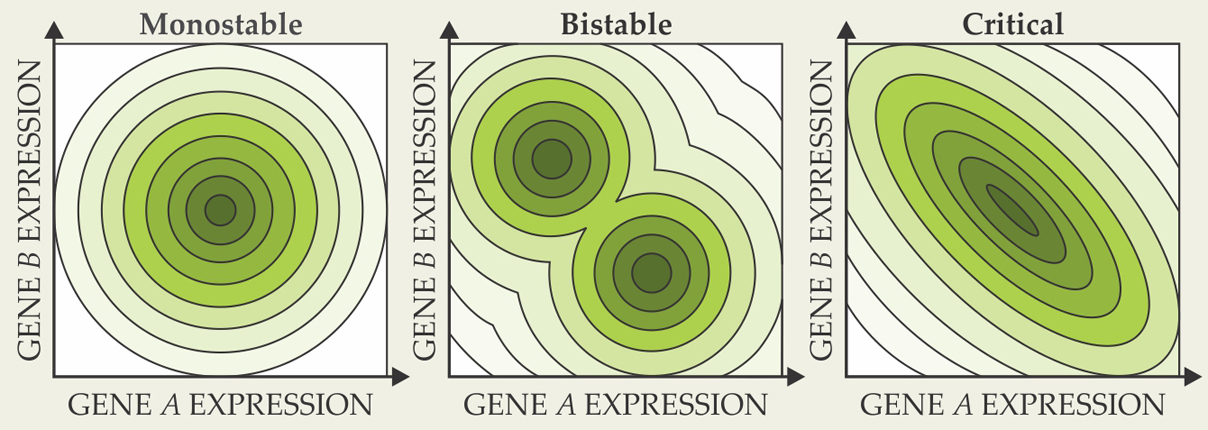
When genes A and B are strongly mutually repressive, the system enters a bistable regime with two steady-state outputs: one in which A is expressed and B is suppressed, and one in which A is suppressed and B is expressed. To switch from one steady-state output to the other, the system must surmount a barrier, characterized by a saddle point on the effective potential surface.

At some intermediate interaction strength, therefore, there must exist a boundary between the monostable and bistable regimes. At that boundary, or critical point, the single potential minimum is on the verge of turning into a saddle point, and the potential surface features a single elongated, flat-bottomed well.

Criticality manifests in several ways. One of them is a strong anticorrelation between fluctuations in g_A and g_B. The system is, more or less, equally likely to be found anywhere at the bottom of the potential well—and less likely to be found outside it—so an increase in g_A is likely to result in a decrease in g_B.

Precision measurements

Until recently, measuring correlations in gene expression fluctuations was impossible. The standard method for measuring gene expression profiles is immunofluorescence: staining a dead tissue sample with a fluorescent antibody that attaches to the protein of interest. Staining a single sample for more than one protein was a challenge, because the antibodies could interfere with each other chemically and because their fluorescence spectra could overlap. And accurate comparisons of protein levels between different specimens were precluded by various sources of systematic error. In the case of the fruit-fly gap genes, two embryos at even slightly different points in their development would have such different expression levels that they’d be impossible to compare.

Gregor and Dubuis developed the first set of fluorescent antibodies to the four main gap genes that could all be used simultaneously. And they developed a new way of measuring the time of embryonic development to within one to two minutes. As a result, they can now measure protein levels, fluctuations, and correlations to within a few percent. ³

Bialek and his colleagues were initially interested in analyzing those measurements to quantify the information conveyed by the gap genes about each cell’s physical position. ⁴ But gradually they realized that they could also learn something about the structure of the gene network itself.

The gap-gene network has four genes, not two, so the simple two-gene picture is of limited use. But there are several regions in the expression profile—shaded in the top panel of figure 2—where just two of the genes have significant expression levels, and the network dynamics are simplified. “Even so,” explains Bialek, “one has to make some perhaps arbitrary choices about the kinds of models one wants to consider.” He and Krotov looked at several possibilities and found that in each case, the model parameters that best fit the data were close to a critical point. “Although we started with specific models, we realized that we could say things in a much more general language. We’ll probably get back to the detailed models at some point.”

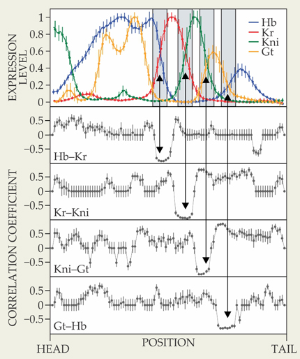
Strong local anticorrelations are a universal feature of a two-gene network at criticality, and indeed, in each of the shaded regions of figure 2, the correlation coefficient between the two active genes approaches −1. Bialek and Krotov identified several other signatures of a two-gene network tuned to a critical point—including slow dynamics, long-range spatial correlations, and non-Gaussian distributions of fluctuations—and found that the gap-gene network exhibits all of them.

Still, they don’t regard their observations as airtight proof that the network is operating at a critical point, because each of the signatures could also arise in other ways. And the implications of criticality (or of a network that mimics one at criticality) are still far from clear. Critical points constitute a small and distinctive region of parameter space, and the odds that a genetic network would find itself near a critical point by chance, from network parameters chosen at random, are small. Then again, life itself occupies a small and distinctive region of parameter space: As Bialek explains, “Most of the ways we can imagine putting molecules in a small box together don’t result in the system organizing itself and walking out of the lab.” Looking further into the question of how and why evolution would guide a system toward critical behavior could, he argues, lead to new insights into what is so special about life. “We take some stabs at this question,” he says, “but we’re still very much in the dark.”

References

1. C. Nüsslein-Volhard, E. Wieschaus, Nature 287, 795 (1980). https://doi.org/10.1038/287795a0
2. D. Krotov et al., Proc. Natl. Acad. Sci. USA 111, 3683 (2014). https://doi.org/10.1073/pnas.1324186111
3. J. O. Dubuis, R. Samanta, T. Gregor, Mol. Syst. Biol. 9, 639 (2013).https://doi.org/10.1038/msb.2012.72
4. J. O. Dubuis et al., Proc. Natl. Acad. Sci. USA 110, 16301 (2013).https://doi.org/10.1073/pnas.1315642110
More about the authors
Johanna L. Miller, jmiller@aip.org