Topological quantum computation

Quantum mechanics is arguably the most successful quantitative theory of nature. The theory is now 80 years old, and no violation of quantum mechanics has ever been detected in any laboratory despite a huge number of experimental tests involving light, atoms, molecules, and solids, as well as nuclei, electrons, and other subatomic particles. In fact, various experimental tests of quantum electrodynamics have achieved an astonishing agreement between measurement and quantum theory—on the order of one part in a billion. Not only is our modern intellectual description of reality entirely quantum mechanical in nature, our modern technology—exemplified by transistors, computer chips, lasers, superconductors, and magnetic storage—is based essentially on underlying quantum phenomena. Solid-state quantum phenomena, in which theory and experiment come together perfectly, have led to voltage standards through the Josephson effect and to resistance standards through the quantum Hall effect.

The recent advent of the concept of quantum computation has opened a new chapter and has spawned serious experimental efforts toward the actual fabrication of a quantum computer. A real-world, commercial quantum computer with, for example, a few million logical quantum bits, or qubits, would enable the efficient solution of computationally difficult problems, such as prime-number factorization and database searching, using the quantum mechanical resources of linear superposition, unitary evolution, and the exponentially large Hilbert space of entangled states. Yet the final read-out process would still be an ordinary classical measurement. In fact, a quantum computer can be exponentially faster than a digital classical computer.

A crucial problem in the construction of a large, many-qubit quantum computer is quantum decoherence: A physical system will remain in a coherent superposition of states only for a finite—often short—time. Any interaction with the rest of the world or any measurement that leads to a “wavefunction collapse” will decohere the system and thereby destroy the encoded quantum information. But a seminal theoretical development underlies the possibility of constructing a quantum computer: quantum error correction, or fault-tolerant quantum computation (see the article by John Preskill in Physics Today, June 1999, page 24 ), which established a threshold theorem that proves that quantum decoherence can be corrected as long as the decoherence is sufficiently weak.

If one thinks of quantum decoherence as unwanted noise in quantum computation, then effective “software” error correction depends on eliminating or minimizing noise in the computer. That approach is similar in spirit to error correction in classical digital computers. For quantum computation, however, an alternative strategy, topological quantum computation, does not try to make the system noiseless, but instead makes it deaf—that is, immune to the usual sources of quantum decoherence. This revolutionary strategy makes quantum decoherence simply irrelevant, thanks to the globally robust topological nature of the computation.

Quantum computation

Suppose we have a controllable quantum system at our disposal. We further assume that it is possible to initialize the system in some known state |ψ ₀〉. We evolve the system by the unitary transform U(t) until it is in some final state |ψ ₁〉 = U(t)|ψ ₀〉. Because that evolution will occur according to some Hamiltonian, we require enough control over the Hamiltonian so that U(t) can be made to be any unitary transformation we desire. Finally, we need a way to measure the state of the system at the end of this evolution.

Such a process of initialization, evolution, and measurement is called quantum computation. ¹ The basic unit of a quantum computer is the qubit—a quantum two-level system with states |0〉 and |1〉—which can be controlled, manipulated, coupled, and entangled with other qubits by external means. The unitary operations themselves define the quantum computational code.

So why hasn’t everyone run out and built a quantum computer? There is a basic obstacle—namely, the occurrence of errors. In the more colorful language of Asher Peres, “Quantum phenomena do not occur in a Hilbert space. They occur in a laboratory.” Of course, errors occur even in classical computers, but they can be surmounted by keeping multiple copies of information and checking against those copies.

With a quantum computer, however, the situation is more complex. If we measure a quantum state during an intermediate stage of a calculation to see if an error has occurred, we may, due to wavefunction collapse, destroy a quantum superposition and thus ruin the calculation. Furthermore, errors need not be merely a discrete bit flip of |0〉 to |1〉, but can be a continuous phase error: $a|0〉+b|1〉\to a|0〉+b{e}^{i\theta }|1〉$ for arbitrary θ. Such continuous errors, superficially reminiscent of errors in classical analog computation, may at first sight appear impossible to rectify; for that reason, quantum computation was long considered to be impossible. In the mid-1990s, however, it was shown that, despite those difficulties, quantum error correction is indeed possible. ¹

One can represent information redundantly so that errors can be identified without measuring the information. However, the error correction process can itself be a little noisy. More errors can then occur during error correction, and the whole procedure will shoot itself in the foot unless the basic error rate is extremely small. Estimates of the threshold error rate above which error correction is impossible depend on the particular error correction scheme, but they typically fall in the range of 10⁻⁴ to 10⁻⁶ (see, for example, reference and references therein). Thus a quantum computer must be able to perform 10⁴ to 10⁶ operations perfectly before an error occurs. That constraint is extremely severe, and although impressive experimental advances have been made over the last five years, it is unclear whether quantum decoherence can be overcome in a practical quantum computer architecture using quantum error correction protocols.

Taming errors is the central physics problem that must be solved for quantum computation to be realized. Topological quantum computation alleviates the problem in a fundamental manner.

Topology and quantum computation

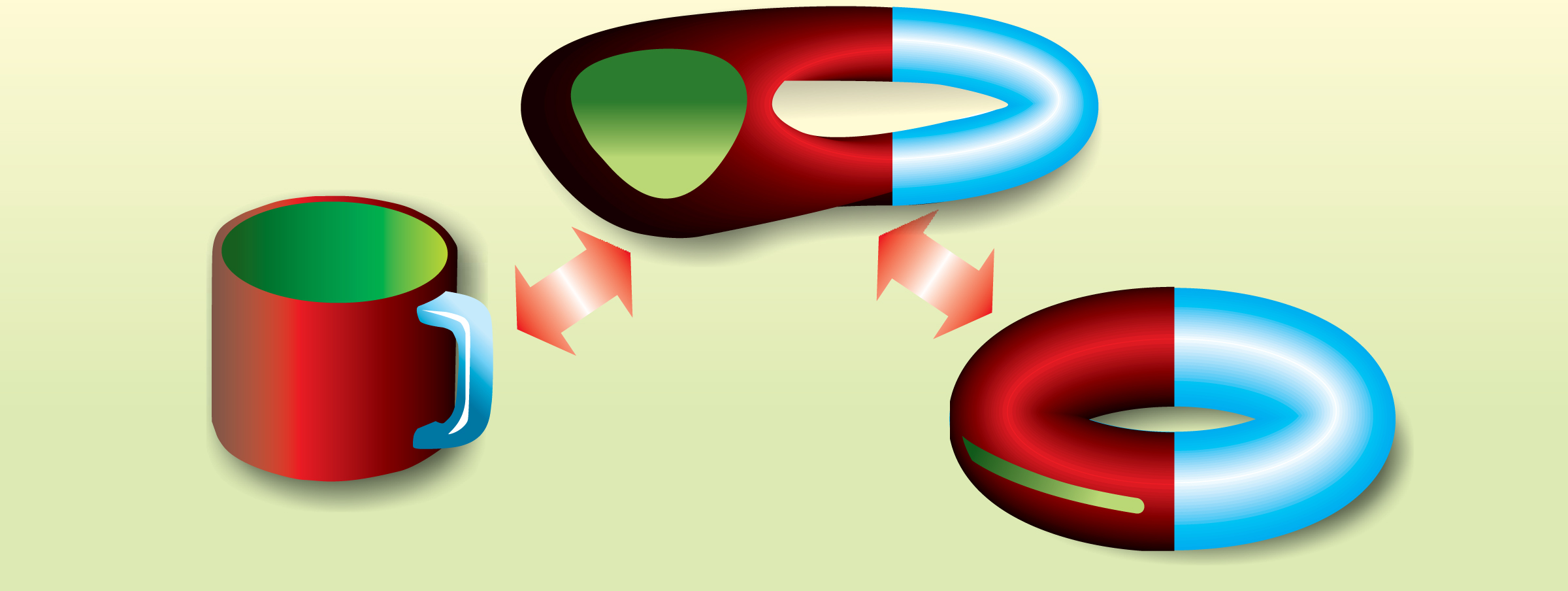
We now seemingly change subjects completely and consider topology, the branch of mathematics concerned with those properties of geometric configurations that are unaltered by elastic deformation. The usual joke is that a topologist cannot tell the difference between a donut and a coffee cup. One can be continuously deformed into the other through a sequence of smooth, small alterations, such as stretching or indenting the surface, without ever tearing it (see figure 1). Both a donut and a coffee cup have a single handle, so each is topologically equivalent to a torus. Topological equivalence can only be destroyed by a drastic change, such as tearing the donut or gluing together two different parts of it. In other words, topology focuses on those features of geometry that are robust against small local perturbations.

Another example of topology is knot theory, which says, for instance, that there is no continuous way to unknot a knotted loop of string. Knot theory is particularly relevant to the physics underlying topological quantum computation. Rather amusingly, similar knot-theory concepts ² also arise in a completely different area of physics, conformal field theory, ³ which has possible applications to string theory.

Local geometry is a highly redundant encoding of topological information. Error correction, though, requires the redundant representation of information so that errors do not occur. Hence, as proposed by Alexei Kitaev, ⁴ if a physical system has topological degrees of freedom that are insensitive to local perturbations, then information contained in those degrees of freedom would be automatically protected against errors caused by local interactions with the environment. If the system happens to be a quantum system, one should, in principle, be able to perform fault-tolerant topological quantum computation without worrying about decoherence—the topological robustness provides quantum immunity.

This idea sounds like the answer to our quest for fault-tolerant quantum computation until we stop for a minute and realize that most physical systems do not have topological degrees of freedom. Instead, they have local degrees of freedom that are sensitive to local perturbations. For instance, if we have a transistor with conductance G and cut out a piece of it, its topology remains intact but we will have drastically affected its conductance G. And for a quantum mechanical spin with two accessible states, the so-called spin qubit, any variation in the local magnetic field will affect the relative phase between those two states. So it doesn’t sound like the topological solution suggested above has anything to do with real-world physics. This pessimistic conclusion is wrong, however, because of one of the most amazing discoveries of the past 30 years.

Topological states of matter

Remarkably, condensed phases of matter do exist that are insensitive to local perturbations. They are topologically invariant at low temperatures and energies and at long distances. These topological states are as real as metals or ordered magnets, but they are not as common.

The existence of such topological states is surprising, since the topological invariance is not a symmetry of the underlying Hamiltonian of electrons and ions that are coupled through the Coulomb interaction in a solid. The Coulomb repulsion between two electrons, and thus the Hamiltonian, depends strongly on the distance between them if the positions of the other electrons and the ions are held fixed (a valid approximation for short time scales). Continuously deforming the system by stretching or contracting it so as to change that distance will affect the energy. Therefore, topological invariance can only be a symmetry that emerges at low energies and long distances. At those scales, as the distance between two electrons is changed by stretching the system, the other electrons will rearrange themselves so as to keep the energy unchanged. In the right circumstances, such invariance could lead to a topological quantum ground state.

Although this idea sounds simple, it is actually a reversal of the paradigm with which many physicists have become accustomed—namely, that low-energy, long-distance physics is less symmetrical than the microscopic equations of motion. In a solid, for instance, the Hamiltonian is invariant under arbitrary uniform translations of all the particles. In the ground state, however, the ions form a crystalline lattice that is invariant under a much smaller group of translations, that is, discrete translations through lattice vectors. The cosmic microwave background provides an example from physics at a very different scale. It has a slight anisotropy, meaning that the temperature is different in different directions, even though the underlying equations are rotationally invariant. Crystalline lattices and the microwave background are both examples of spontaneously broken symmetry.

Topological states of matter are an example of the converse: physical systems in which the low-energy, long-distance physics is more symmetrical than the microscopic equations. This is emergent symmetry.

In more technical language, we would say that a system is in a topological phase if its low-energy, long-distance effective field theory is a topological quantum field theory—that is, if all of its physical correlation functions are topologically invariant up to corrections of the form e ^–Δ/T at temperature T for some nonzero energy gap Δ. This behavior is precisely what is found in the fractional quantum Hall effect, ⁵ as discussed in box 1.

Anyons and braiding

In addition to their fractional charge (see box 1), quasiparticles in the fractional quantum Hall effect have another remarkable property: They are anyons. Anyons were first proposed as a mathematical possibility in which any phase factor e ^iα , not just +1 for bosons and −1 for fermions, can result from a counterclockwise interchange of two particles. Such natural generalizations of fermions and bosons are topologically allowed in two spatial dimensions. To understand anyons a little better, we first look at the braiding of particle trajectories in two spatial dimensions.

Consider the braiding properties of particle trajectories in 2 + 1 dimensions (2 spatial and 1 time dimension). According to Richard Feynman’s path-integral formalism, the quantum mechanical amplitude for n particles that are at positions x ₁, x ₂, …, x_n at an initial time t ₀ to return to those coordinates at a later time t is given by a sum over all trajectories. Each trajectory is summed with weight e ^iS/ħ , where S is the trajectory’s classical action. This particular assignment of weights is consistent with the classical limit: As ħ → 0, the stationary points of the action dominate and give the familiar classical solutions. A peculiarity of two spatial dimensions, however, is that the space of particle trajectories is disconnected: As may be seen in figure 2, it is not always possible to continuously deform a given trajectory into a different one.

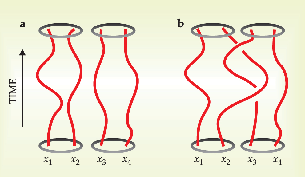
Consequently, at the quantum mechanical level, we have the freedom to weight each trajectory’s contribution to the path integral by a different phase factor. Since the trajectories are not continuously deformable into each other, the classical limit is completely blind to the phases we choose.

These phase factors constitute an abelian (commutative) representation of the braid group. For the case of two particles, the braid group is simply the group of integers, with integer n corresponding to the number of times one particle winds counterclockwise about the other (negative integers are clockwise windings). If the particles are identical, then we must allow exchanges as well, which we can label by half-integer windings. The different representations of the braid group of two identical particles are labeled by a phase α, so that a trajectory in which one particle is exchanged counterclockwise with the other n times receives the phase factor e^inα.

If α = 0, the particles are bosons; if α = π, the particles are fermions. For intermediate values of α, the particles are anyons. The anyonic representations of the braid group are just an extension of the two-particle case: Whenever any of N identical particles is exchanged counterclockwise n times with another, the system gains a phase factor e^inα.

In interacting many-body systems—such as metals, semiconductors, magnets, and liquid helium—the low-energy excitations that control most of the observable properties behave, somewhat magically, much like weakly interacting particles. Such excitations, dubbed quasiparticles by Lev Landau, are usually bosons or fermions. However, in a fractional quantum Hall state—and perhaps elsewhere—quasiparticle excitations above the ground state are anyons. In the fractional quantum Hall state with filling factor $v=\stackrel{1}{}/\underset{3}{}$ , for example, a phase e ^2πi/3 results when one quasiparticle encircles another; when a counterclockwise exchange occurs, half of that phase is accrued, e ^πi/3. In fact, the phase factor is exactly e ^2πi/3, independent of shape, speed, and other trajectory details. Finite-temperature corrections to the phase changes are on the order of e ^–Δ/T , as in longitudinal and transverse resistance in the Hall regime (see box 1). At low temperatures, those corrections are extremely small.

Abelian anyons provide an example of a unitary transformation that can be performed exactly in a topological state of matter. Unfortunately, it is a trivial transformation, just changing the phase of the wavefunction. To apply unitary transformations that are useful for quantum computation, we will need a special class of topological states that support non-abelian anyons.

Non-abelian anyons

Abelian anyons at the $\raisebox{1ex}{$1$}\!\left/ \!\raisebox{-1ex}{$3$}\right.$ fractional quantum Hall state do not constitute the most exotic possibility that one can imagine. Suppose we have g degenerate states ψ_a , where a = 1, 2, …, g, of particles at positions x ₁, x ₂, …, x_n. Exchanging particles 1 and 2 might do more than just change the phase of the wavefunction. It might rotate it into a different one in the space spanned by the ψ_a states. Expressed in terms of those states, ψ_a → M_ab ψ_b. Exchanging particles 2 and 3 may lead to a different rotation: ψ_a → N_ab ψ_b.

If M_ab and N_ab do not commute—that is, if M_abN_bc ≠ N_abM_bc —the particles are said to obey non-abelian braiding statistics. With such particles, we can effect nontrivial unitary transformations just by braiding particles. Thus, non-abelian quasiparticles are the sine qua non for topological quantum computation.

Non-abelian braiding gives the answer to a question that may have been bothering the reader: If topological protection is so effective at isolating quantum information from errors caused by the environment, how can we manage to manipulate and read the information? If the quasiparticles of the system exhibit non-abelian braiding statistics, that is, if they are non-abelian anyons, then the g-dimensional Hilbert space of n-particle states can be used to store quantum information. To manipulate it, we need to perform braiding operations on the n quasiparticles in the system. Ideally, we would like to be able to perform any desired unitary transformation (or at least to approximate it within desired accuracy) simply by braiding quasiparticles. For a large class of states, such manipulation can indeed be done. ⁶ At the end of a calculation, we can read the state of the system by using a non-abelian generalization of the Aharonov–Bohm effect to make a topological measurement of topological information: By sending in a non-abelian anyonic test quasiparticle and allowing its different trajectories to encircle the quasiparticles that contain the desired quantum information, we can read that information through the quantum interference between the trajectories.

To explore how non-abelian braiding could work, consider two simple models. The first model has three basic quasiparticle types, which we’ll label 0, $\raisebox{1ex}{$1$}\!\left/ \!\raisebox{-1ex}{$2$}\right.$ , and 1. These three labels are the “topological charges”—essentially a generalization of the α phase factors—of the three quasiparticle types. An arbitrary combination of quasiparticles can similarly be labeled by a topological charge. In an abelian system, the total charge is simply the sum of each quasiparticle’s charge. But in a non-abelian system, the addition rules get complicated; in this first model, the rules resemble those for quantum mechanical angular momenta.

We’ll say a quasiparticle of charge 0 is present when the system is in its ground state—that is, when no quasiparticles are present at all. It is also possible for a collection of nonzero quasiparticles—like quantum mechanical spins—to essentially cancel each other out, so that when another quasiparticle is taken around the entire collection, nothing happens. In that case, we again say that the collection has total topological charge 0. Alternatively, the topological charge of a collection could be $\raisebox{1ex}{$1$}\!\left/ \!\raisebox{-1ex}{$2$}\right.$ or 1. These are the only possibilities. If we consider, for example, two $\raisebox{1ex}{$1$}\!\left/ \!\raisebox{-1ex}{$2$}\right.$ quasiparticles, their total topological charge can be either 0 or 1. However, if we have two 1 quasiparticles, their total topological charge must be 0, and if we have a $\raisebox{1ex}{$1$}\!\left/ \!\raisebox{-1ex}{$2$}\right.$ and a 1, their total topological charge must be $\raisebox{1ex}{$1$}\!\left/ \!\raisebox{-1ex}{$2$}\right.$ . (The combination of 0 and any j is j.)

Suppose we have four quasiparticles of type $\raisebox{1ex}{$1$}\!\left/ \!\raisebox{-1ex}{$2$}\right.$ whose total topological charge is 0. The total topological charge of the first and second quasiparticles can be either 0 or 1. If it is 0, then the total topological charge of the third and fourth must also be 0 since the total of all four is 0. Similarly, if the topological charge of the first two is 1, then that of the third and fourth must also be 1. Thus, we have two states of four $\raisebox{1ex}{$1$}\!\left/ \!\raisebox{-1ex}{$2$}\right.$ quasiparticles and, continuing in a similar manner, 2 ⁿ⁻¹ states of 2n quasiparticles of type $\raisebox{1ex}{$1$}\!\left/ \!\raisebox{-1ex}{$2$}\right.$ for which the total topological charge is 0.

These arguments suggest a way to create a basis to describe this degenerate space of states. Combine the 2n quasiparticles into n pairs. Each pair can have a topological charge of 0 or 1; only the charge of the last pair is constrained, since the total charge of all 2n quasiparticles is 0. Thus, 2n quasiparticles form n − 1 qubits. An arbitrary state of the system can be projected onto basis states formed by assigning a definite charge of 0 or 1 to each qubit; each basis state thus corresponds to a sequence of n − 1 classical bits.

In such a basis, the braiding rules are as follows. When two quasiparticles belonging to the same pair are braided, a basis state only changes by a phase. However, when a quasiparticle from pair i is taken around a single quasiparticle from pair j, as in figure 2(b), a NOT gate is applied to qubits i and j (up to a phase). When a quasiparticle is taken around both quasiparticles in pair j, a basis state is multiplied by +1 if bit j has charge 0, and by −1 if the bit has charge 1. Therefore, the two braiding operations between pairs do not commute. From these braiding rules we can determine the effect of an arbitrary braid on any initial state. Unfortunately, braiding alone is insufficient in this system to generate all possible unitary transformations. However, the next example is sufficient and therefore supports universal quantum computation through braiding. ⁶

Now consider a model with only a single nontrivial quasiparticle type, with topological charge 1. As before, it is useful to say that a quasiparticle of charge 0 is present when no quasiparticles of charge 1 is present. When two quasiparticles are present, their combined state can be either 0 or 1. Suppose we have n quasiparticles with total topological charge 0; let A_n be the number of such states. To determine A_n , pick two of the quasiparticles. Their combined state is either 0 or 1. If their combined state is 0, then the remaining n − 2 quasiparticles must also have total topological charge 0, and there are A _n−2 of those states. If the combined topological charge of the two quasiparticles is 1, then the pair is topologically equivalent to a single quasiparticle of charge 1, and so the system behaves as if there were n − 1 quasiparticles of type 1; there are A _n−1 of those states that have total charge 0. Hence, A_n = A _n−1 + A _n−2. The dimension of the Hilbert space for n + 1 particles is thus the nth Fibonacci number, and these quasiparticles are sometimes called Fibonacci anyons.

For an example of their braiding rules, consider four quasiparticles whose total topological charge is 0. If we divide the quasiparticles into two pairs, each pair can have a total topological charge of either 0 or 1; thus we can label the two states |0〉 and |1〉. If the initial state is |0〉, then detailed calculations show that the braid of figure 2(b) transforms it to τ ⁻² (τe ^4πi/5 + e ^2πi/5) |0〉 + τ ^−3/2 (e ^πi/5 − e ^3πi/5) |1〉, where τ = τ ² − 1 is the golden ratio, $(1+\sqrt{5})/2$.

In the first example, braiding operations had the effect of ^π/₂ rotations about orthogonal axes in Hilbert space; such rotations form a finite group. In the second example, however, the rotations are by multiples of ^π/₅ about different axes in Hilbert space. Those rotations do not form a finite group but rather a dense set, so any desired unitary transformation can be approximated to arbitrary accuracy. Thus, Fibonacci anyons support universal quantum computation. ⁶ Reference presents specific gates for such non-abelian anyons.

Now all we need is to identify a stable topological state supporting quasiparticles that are non-abelian anyons and then perform the requisite braiding operations to carry out topological quantum computation.

Non-abelian topological phases in nature

The most likely known candidate ^8,9 for finding a topological state with non-abelian anyonic excitations is the fractional quantum Hall state at the plateau observed at $v=\stackrel{5}{}/\underset{2}{}$ . Quasiparticle excitations (which, according to theory, have charge ^e /₄) about this ground state are suspected to be non-abelian anyons ^10,11 of precisely the type discussed in the first example above.

How can we tell experimentally if this hypothesis is correct? How can we use this state for quantum computation? These two questions have essentially the same answer: By performing braiding operations and observing their effects, we can deduce the non-abelian statistics of the quasiparticles in the state and apply fault-tolerant quantum gates to topologically protected qubits. Recent theoretical work ¹²⁻¹⁵ proposes specific experiments to achieve these two ends, as described in box 2.

The $v=\stackrel{5}{}/\underset{2}{}$ state, if it is non-abelian, would realize the braiding statistics of the first example above. But those braiding operations alone cannot implement any desired unitary transformation. To achieve that completeness, quasiparticle braiding must be supplemented by either some unprotected operations or some other topological operations, such as topology change. However, the $v=\stackrel{12}{}/\underset{5}{}$ quantum Hall state, if it is non-abelian, would most likely realize the non-abelian statistics of the second example in the previous section, and thus could support universal topological quantum computation.

A non-abelian quantum Hall state is currently the most promising route to topological quantum computation and perhaps the most promising route of any kind to scalable, fault-tolerant quantum computation. However, we should also look elsewhere for a topological quantum computer, even though that search requires reinventing the wheel that is already in motion in the context of the fractional quantum Hall effect. We need to understand how and when topological phases can occur in other physical systems. Some possibilities are p-wave superconductors such as strontium ruthenate ¹⁶ (see Physics Today, January 2001, page 42 ), frustrated quantum magnets ¹⁷ (see Physics Today, February 2006, page 24 ), and cold atoms in optical lattices ¹⁸ (see Physics Today, March 2004, page 38 ). Where to find such phases is very much an open problem. One might be only half-joking in suggesting that the easiest way to solve that problem might be to build a fractional quantum Hall quantum computer first and then use it on the solid-state physics problems that must be solved to develop a “high-temperature” topological quantum computer.

Outlook

The most important issues facing topological quantum computation are twofold: (1) finding or identifying a suitable system with the appropriate topological properties (that is, non-abelian statistics) to enable quantum computation; and (2) figuring out a scheme to carry out the braiding operations necessary to achieve the required unitary transformations. Both are tall orders, and any experimental progress even in accomplishing the first one would be an important achievement.

The only topological system definitely known to exist in nature is in the quantum Hall regime, where topological states, such as the $v=\stackrel{1}{}/\underset{3}{}$ fractional quantum Hall state, that support abelian anyonic excitations are reasonably well established. Of course, for topological quantum computation, anyons are necessary but not sufficient. We also need non-abelian anyonic statistics, which may exist in the observed $v=\stackrel{5}{}/\underset{2}{}$ fractional quantum Hall state. The reason for discussing the fractional quantum Hall state at length in this article is precisely because it is the only known concrete candidate that addresses both of the above issues. One cannot, however, rule out the possibility that the $\raisebox{1ex}{$5$}\!\left/ \!\raisebox{-1ex}{$2$}\right.$ state is not non-abelian, since currently there is, at best, only indirect experimental and theoretical evidence that it is non-abelian.

The good news is that experiments are under way to test the non-abelian nature of the quasiparticle statistics in the $\raisebox{1ex}{$5$}\!\left/ \!\raisebox{-1ex}{$2$}\right.$ state (see box 2). But even if the $\raisebox{1ex}{$5$}\!\left/ \!\raisebox{-1ex}{$2$}\right.$ state is definitively shown to be a non-abelian state, it is still not enough for a universal quantum computer. It can form a perfect quantum memory, but it does not allow any general unitary transformation to be applied.

The state with $v=\stackrel{12}{}/\underset{5}{}$ is extremely fragile and is barely observable even at low temperatures (on the order of 20 mK) and in the best samples. ⁹ It may be a non-abelian state that supports universal quantum computation. However, much is unknown about the $\raisebox{1ex}{$12$}\!\left/ \!\raisebox{-1ex}{$5$}\right.$ state, and its possible role in topological quantum computation is speculative at this stage.

Thus there is a strong need to find other systems satisfying the above two criteria for topological quantum computation. Although a few non-quantum-Hall proposals have been put forth, concrete suggestions for how to carry out quasiparticle braiding exist only in quantum Hall systems. Yet even unsuccessful quests for other systems capable of supporting topological quantum computation will likely reap rewards along the way.

References

1. J. Preskill, Lecture Notes in Quantum Computation, http://www.theory.caltech.edu/people/preskill/ph229/#lecture .
2. V. F. R. Jones, Bull. Am. Math. Soc. 12, 103 (1985) https://doi.org/10.1090/S0273-0979-1985-15304-2 .
3. E. Witten, Commun. Math. Phys. 121, 351 (1989) https://doi.org/10.1007/BF01217730 .
4. A. Kitaev, Ann. Phys. (NY) 303, 2 (2003) https://doi.org/10.1016/S0003-4916(02)00018-0 .
5. S. Das Sarma, A. Pinczuk, eds., Perspectives in Quantum Hall Effects: Novel Quantum Liquids in Low-Dimensional Semiconductor Structures, Wiley, New York (1997).
6. M. H. Freedman, M. Larsen, Z. Wang, Commun. Math. Phys. 227, 605 (2002) https://doi.org/10.1007/s002200200645 .
7. N. E. Bonesteel et al., Phys. Rev. Lett. 95, 140503 (2005) https://doi.org/10.1103/PhysRevLett.95.140503 .
8. R. L. Willett et al., Phys. Rev. Lett. 59, 1776 (1987) https://doi.org/10.1103/PhysRevLett.59.1776 .
9. J. S. Xia et al., Phys. Rev. Lett. 93, 176809 (2004) https://doi.org/10.1103/PhysRevLett.93.176809 .
10. G. Moore, N. Read, Nucl. Phys. B 360, 362 (1991) https://doi.org/10.1016/0550-3213(91)90407-O .
11. C. Nayak, F. Wilczek, Nucl. Phys. B 479, 529 (1996) https://doi.org/10.1016/0550-3213(96)00430-0 .
12. E. Fradkin, C. Nayak, A. M. Tsvelik, F. Wilczek, Nucl. Phys. B 516, 704 (1998) https://doi.org/10.1016/S0550-3213(98)00111-4 .
13. S. Das Sarma, M. Freedman, C. Nayak, Phys. Rev. Lett. 94, 166802 (2005) https://doi.org/10.1103/PhysRevLett.94.166802 .
14. A. Stern, B. I. Halperin, Phys Rev. Lett. 96, 016802 (2006) https://doi.org/10.1103/PhysRevLett.96.016802 .
15. P. Bonderson, A. Kitaev, K. Shtengel, Phys Rev. Lett. 96, 016803 (2006) https://doi.org/10.1103/PhysRevLett.96.016803 .
16. S. Das Sarma, C. Nayak, S. Tewari, http://arXiv.org/abs/cond-mat/0510553 .
17. A. Kitaev, http://arXiv.org/abs/cond-mat/0506438 .
18. L.-M. Duan, E. Demler, M. D. Lukin, Phys. Rev. Lett. 91, 090402 (2003) https://doi.org/10.1103/PhysRevLett.91.090402 .
More about the authors
Sankar Das Sarma is a Distinguished University Professor at the University of Maryland, College Park, and director of the university’s condensed matter theory center. Michael Freedman is director of Microsoft Project Q at the University of California, Santa Barbara. Chetan Nayak is a senior researcher at Microsoft Project Q and a professor in the department of physics and astronomy at the University of California, Los Angeles.
Sankar Das Sarma, 1 University of Maryland, College Park, US .
Michael Freedman, 2 University of California, Santa Barbara, US .
Chetan Nayak, 3 University of California, Los Angeles, US .