The geodynamo’s unique longevity

Exploration of the solar system has confirmed that most of its planets have magnetic fields. Although the planets differ in important details, the reason they are magnetic is fundamentally the same: In each planet, a self-sustaining dynamo has operated at some time in history. In such a dynamo, electric currents and magnetic fields are continuously induced by motions of conducting fluid inside the planet.

The evidence for self-sustaining dynamo action throughout the solar system—Venus may be the lone planetary exception—is not surprising because only three basic ingredients are needed: a large volume of electrically conducting fluid, planetary rotation, and an energy source to stir the fluid. Planets generally acquire all three in abundance during their formation. Indeed, dynamo action is not limited to the planets; it produces the 11-year solar cycle, ¹ and evidence exists for dynamo action in the Moon, in some of the Galilean satellites, and even in meteorite parent bodies. ²

More puzzling, however, is the fact that other terrestrial (that is, solid) planets and satellites failed to sustain dynamo action for very long. In Mars and the Moon, the record of remnant crustal magnetization points to dynamo cessation within a few hundred million years after their formation. ³ The geodynamo, on the other hand, managed to locate a fountain of youth that its sibling planets had missed, and it is still going strong. (Earth is 4.54 billion years old.) The geomagnetic field intensity is actually greater today than at most times in the past, even though its intensity happens to be rapidly decreasing at the moment. Furthermore, over the past 5 million years, the geomagnetic field has reversed polarity at near-record rates, a sure sign of vigor.

What accounts for such stark differences in the dynamo histories of otherwise similar planets? Both Mars and Venus rotate and have large metallic cores, comparable to Earth, so the answer is not likely to be found in those features. Instead, it appears that Earth’s core has tapped into a much larger reservoir of energy, sufficient to power the geodynamo for billions of years, with no end in sight. The cores in some other terrestrial planets were forced to operate on far leaner energy budgets, and rather quickly those budgets proved too austere.

Heating and cooling

Current models of solar-system formation emphasize the important influence of large impacts on the initial structure and state of the terrestrial planets and on the process of core formation, ⁴ which is likely when dynamo action began. Giant impacts are thus a good place to look for the source of differences between terrestrial planets. The impacts produce copious melting and allow core-forming metals (mainly iron and nickel) to quickly and efficiently segregate from mantle-forming silicates within superheated magma oceans. (See the article by Bernard Wood, Physics Today, December 2011, page 40 .)

That scenario applies particularly well to early Earth in light of the hypothesized impact of a Mars-sized object that produced the Moon (see the article by Robin Canup, Physics Today, April 2004, page 56 ). Earth’s newly formed core would have been very hot—well over 5000 K and totally molten—replete with lighter elements such as oxygen, sulfur, silicon, and perhaps magnesium and carbon. As Earth’s core cooled over geologic time, its composition necessarily changed. The iron–nickel mixture that makes up most of the core likely became saturated with respect to the least-soluble light elements; those accumulated at the top of the core and possibly became incorporated into a remnant magma ocean at the base of the overlying mantle, as illustrated in figure 1.

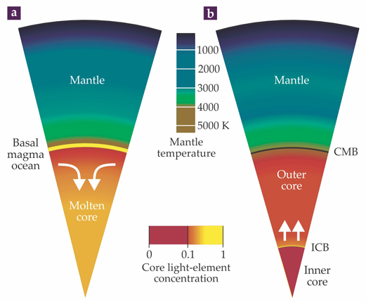
The dense residual liquid metal, partially depleted of lighter elements, sank back into the core and in doing so produced the motions needed to induce the electric currents for the early geodynamo. The duration of that first stage of the dynamo’s evolution is unknown, but it may well have lasted several billion years. With additional cooling, the liquid metal in the core eventually reached its solidification temperature. Solidification probably started at Earth’s center: The melting temperature of iron-rich alloys increases so rapidly with pressure that most terrestrial cores are expected to freeze from the inside out. With solidification, Earth’s core entered a second phase of evolution. And further cooling has led to the progressive growth of the solid inner core to its present size—the final major step in the construction of our modern planet. ⁵

According to the above model, the solid inner core forms rapidly and therefore may be relatively young. The present-day heat loss from the entire core is uncertain, but best estimates ⁶ place it in the range of 10–16 TW (by comparison, the total heat loss from Earth’s interior—crust, mantle, and core—is approximately 46 TW). The solidification rate of the inner core is thus about 6000 Mg/s if we ignore radioactive heat sources. Extrapolating backward in time to first nucleation, the predicted age of the inner core is less than 1 billion years, far younger than Earth itself. Only a large dose of radioactive heat in the core—the isotope potassium-40 being the most likely source—would prevent the inner core from solidifying so quickly.

An important property shared by both evolutionary stages in figure 1 is that the gravitational potential energy of the core decreases. As described in the companion article by Bruce Buffett on page 37 , that release of gravitational potential energy and its conversion to kinetic energy of fluid motion are primarily what has sustained the geodynamo over its long history. During the first stage, the density of the core increased by thermal contraction and the loss of insoluble light elements. During the second stage, which is ongoing, thermal contraction continues. But more importantly, soluble light elements are being concentrated in the liquid outer core and depleted from the solid inner core. The result is that the density of the outer core drops while the density of the inner core rises. In both stages, the partitioning of light elements leads to unstable stratification, which produces in the fluid convective motions that redistribute the light elements and lower the gravitational potential energy of the core as a whole. Ordinary electromagnetic induction then converts part of the kinetic energy of fluid motion into electromagnetic (mostly magnetic) energy, which completes the dynamo process.

Alternative energy sources—for example, instabilities produced by Earth’s precession and tidal forces—may contribute additional power. Radioactive heat sources may also contribute to the overall energy balance in the core. But the gravitational dynamo mechanism is thought to provide most of the power for the geodynamo, ⁷ and accordingly, the future of the geodynamo is particularly bright. As of today, only about 4% of Earth’s core has solidified, so there is plenty of energy remaining to sustain the geomagnetic field for hundreds of millions, if not billions, of years to come.

The mantle matters

Why then has the dynamo process not been sustained in other terrestrial planets? The probable answer lies beyond the dynamo region in the solid silicate mantle that surrounds the metallic core of each planet. Earth’s mantle is unique among terrestrial planets in that it supports a global system of plate tectonics. The creeping flow of the silicate material associated with plate motions overturns Earth’s mantle on time scales of tens of millions to hundreds of millions of years. The flow efficiently draws heat off the core–mantle boundary and transports it to the surface within giant upwellings and plumes. Without the heat transport provided by mantle flow, the cooling rate of Earth’s core would be vastly reduced, and so would be the strength of the dynamo mechanism.

It’s an open question why plate tectonics are absent from other terrestrial planets. According to one hypothesis, mobile plates require water-filled oceans because water weakens mantle rocks and plate boundaries (see the article by Marc Hirschmann and David Kohlstedt, Physics Today, March 2012, page 40 ). Another hypothesis is that surface temperature controls plate formation. ⁸ In any case, without mobile plates—and in particular, without plate subduction—mantle overturn is weak, intermittent, or nonexistent. Consequently, long-term sustainable dynamo action in a terrestrial planet without subduction becomes uncertain.

The criterion that best distinguishes a sustainable fluid dynamo from an unsustainable one is the magnetic Reynolds number Rm. An often-used definition of that parameter is Rm = μσud, where μ is magnetic permeability of the fluid, σ is its electrical conductivity, u is the root-mean-squared fluid velocity, and d is the depth of the dynamo region. In physical terms, Rm is the ratio of two fundamental time scales: the decay time of electric currents due to ohmic resistance in the fluid divided by the characteristic time for fluid circulation. Dynamo action requires a large Rm. However, that can be achieved in multiple ways. For example, laboratory dynamos reach large magnetic Reynolds numbers using high fluid velocities, whereas planetary dynamos reach them by virtue of large fluid depths.

Theory, laboratory experiments, and numerical simulations show that the critical Rm for dynamo action is about 40. The Rm of the geodynamo can be estimated by measuring the electrical conductivity of core alloys at high pressure and high temperature and by inferring the fluid velocity from spacecraft measurements that track the motion of geomagnetic field lines emanating from the core. Because magnetic field lines move with the fluid where Rm is high, tracking the variation of the geomagnetic field traces the fluid motion in the outer core. That approach yields Rm between 1000 and 2000, well above the critical value. ⁹ The relatively fast flow speeds of nearly 1 mm/s in Earth’s outer core may be far greater than in other terrestrial planets because their mantles, lacking plate tectonics, are less efficient at heat transport. Indeed, the simplest explanation for why some planetary dynamos failed quickly is that heat transport in their mantles became too low to maintain supercritical Rm conditions in the core.

Magnetic induction by flow

The box on the left illustrates the basic form of convection and dynamo action in Earth’s outer core as they are currently envisioned. Theory, laboratory experiments, numerical simulations, and geomagnetic observations are in fundamental agreement that convection in the outer core consists of vortices aligned in the direction of the rotation axis. The alignment is a consequence of the dominance of the Coriolis acceleration and is an expression of the so-called Taylor–Proudman constraint familiar in rotating fluid mechanics.

Columnar convection is particularly efficient at dynamo action because of a kinematic property called helicity, which, simply put, corresponds to the flow of fluid parcels along helical paths. As described in the box, the helical flow of molten iron allows for the induction of a toroidal magnetic field from a poloidal magnetic field and vice versa. The helical flow thus provides the positive feedback between the two magnetic field components that is essential for dynamo action. The sign of helicity is also significant, being generally negative in the northern hemisphere of the core and positive in the southern hemisphere. The antisymmetry is the primary reason why the geomagnetic pole, when averaged over time, tends to coincide with Earth’s rotation axis.

Flipping fields

In addition to sustaining Earth’s magnetic field, the geodynamo’s supercritical state is responsible for polarity reversals. As figure 2a illustrates, reversals have occurred throughout history, although with a highly variable frequency. The recent geomagnetic field has reversed rather frequently on average—about four times per million years—despite the fact that the current polarity epoch, the Brunhes chron, has persisted for about 780 000 years.

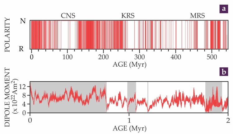
Figure 2 also shows that three times in the current era the geomagnetic field basically stopped reversing for tens of millions of years—periods known as geomagnetic superchrons. Further into the past the geomagnetic record becomes increasingly sketchy; even so, evidence suggests that the alternation between reversing and nonreversing behavior has characterized the geodynamo for a very long time.

Polarity reversals of the solar dynamo occur every 11 years, almost like clockwork. In contrast, reversals of the geodynamo are more widely spaced in time and occur far less regularly. The consensus view is that geomagnetic reversals have their origin in perturbations in the magnetic field of the core, rather than in external disturbances. But unlike the solar dynamo, reversals are not essential to the geodynamo process. Instead, frequent reversals indicate that the core is “overpowered” compared with its average state, and superchrons indicate that the core is “underpowered.”

That interpretation is supported by systematic investigations of the polarity reversal process using first-principles numerical dynamo models, ¹⁰ which show that although the timing of individual reversals is basically random, physical factors influence their likelihood. For example, increasing the angular velocity of planetary rotation tends to stabilize dynamo magnetic fields against polarity reversal, whereas increasing the vigor of convection tends to have the opposite effect. An increase in large-scale shear flow also often tends to increase the likelihood of a reversal.

Figure 3 illustrates a reversal in a simulated dynamo through a series of snapshots, each separated by 4000 years. Initially, as shown in column a, the radial magnetic field intensity on the core–mantle boundary is strongly positive, as is the axial dipole moment of the field. The reversal process begins in a region of the core where convection happens to be particularly vigorous and magnetic field lines experience anomalously large amounts of twisting and bending by virtue of the high rates of strain in the fluid motion—enough bending to locally reverse the magnetic field direction. The blue-colored magnetic field lines in the middle row reveal one locally reversed region.

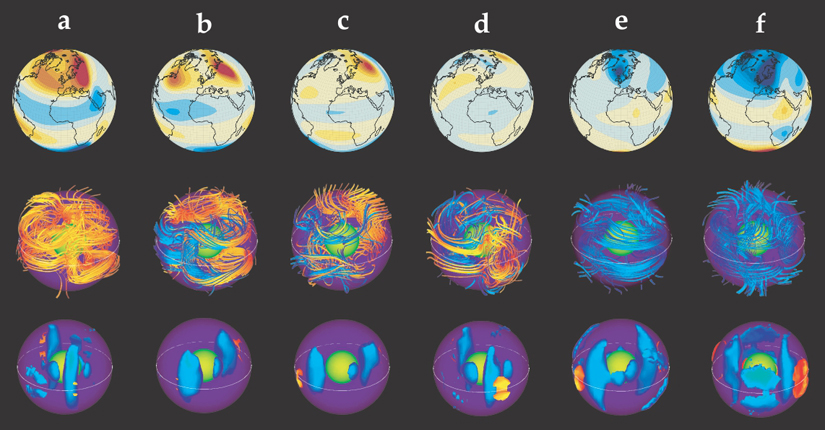
Because the fluid velocities are somewhat higher in that region, the local Rm may be higher as well compared with the rest of the core. And if conditions for growth are favorable, the reversed magnetic field there will intensify faster than in surrounding regions. Under those circumstances, the reversed field expands and occupies an increasingly larger portion of the core until the polarity of the magnetic field inside the core becomes mixed, as in columns c and d, and it leads to a sharp drop in the magnitude of the geomagnetic dipole moment, normally the dominant and most stable component of the external geomagnetic field.

What remains of the external field after dipole collapse is a low-intensity, spatially complex superposition of the weak dipole plus higher-harmonic components, the so-called transition field. What happens next depends on poorly understood details of the way the dipole field regenerates. It could regenerate with its old polarity, completing what’s called a polarity excursion. Or it could emerge with the opposite polarity and complete the reversal.

Evidence of reversals

Geomagnetic reversals and excursions can usually be identified on the basis of rock magnetization alone, because to a good approximation, the directions of the magnetization before and after the reversal correspond to the directions produced by an axial dipole. In contrast, variations in geomagnetic intensity are far more difficult to extract from the rock record.

Nevertheless, geomagnetic intensity variations obtained from the magnetization of deep ocean sediments provide dramatic evidence of the reversal process. Figure 2b offers a two-million-year reconstruction of the variations of the geomagnetic dipole moment derived from magnetized ocean sediments worldwide. The quantity shown is called the virtual axial dipole moment, because the field model used to interpret the sediment magnetization consists of just an axial dipole. The figure shows that the dipole intensity drops by a factor of five or more over several thousand years prior to reversal and then recovers on approximately the same time scale, if not slightly faster. It also shows that for every successful reversal, there are several excursion events in which the dipole moment dropped substantially but has returned to its old polarity.

The behavior of the modern geomagnetic field offers clues to how the reversal process may begin. Ever since the first measurements by Carl Friedrich Gauss early in the 19th century, the geomagnetic dipole moment has been in steep decline, losing intensity at a rate of nearly 6% per century. That’s about 20 times as fast as free decay, the rate at which the field would decrease by ohmic resistance were the dynamo to shut off. Indeed, it is sometimes said that we live in an “antidynamo” era. However, the evidence suggests that magnetic energy in the dipole field is actually being transferred—cascading up the geomagnetic spectrum to higher-multipole field components, precisely the action that causes dipole collapse in numerical dynamos.

Figure 4a shows a map of the modern geomagnetic field at the core–mantle boundary, the top of the active dynamo region. It was made from satellite magnetic field measurements extrapolated down to the core boundary on the assumption that the mantle is an insulator. The map reveals that the axial dipole, which dominates the geomagnetic field outside the core, emanates from a handful of high-intensity patches, two of which appear aligned roughly along longitudes 90° E and 110° W and are suggestive of the columnar symmetry expected for convection in the outer core. There is much nondipole structure in figure 4a—particularly in regions where the field has reversed polarity. Such locally reversed regions now cover a substantial fraction of the core–mantle boundary, and their sudden development over the past few hundred years largely accounts for the observed rapid decrease in the geomagnetic dipole moment.

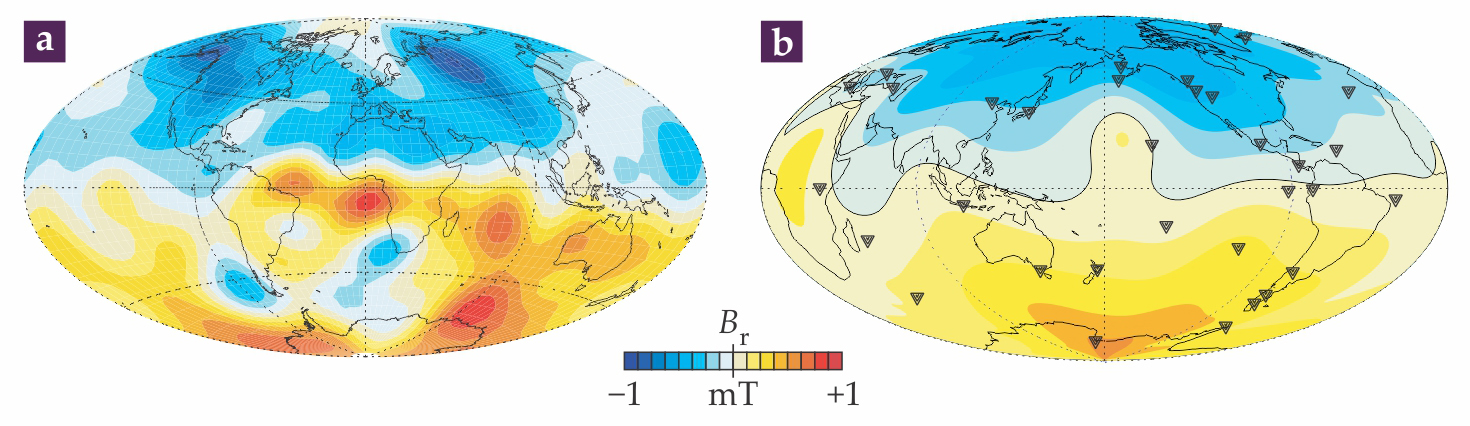
For interpreting the geodynamo, it is important to distinguish transient structures in the modern geomagnetic field from those that are long lasting. Figure 4b shows a map of the geomagnetic field derived from paleomagnetic measurements averaged over the past 5 million years. The axial dipole field is even more dominant in that map than in the modern snapshot. Yet significant nonaxial structure persists, especially in the northern hemisphere, where the two high-intensity flux patches are smeared out into high lobes separated by a relatively weak field beneath the Pacific Ocean and Africa.

The significance of the nonaxial structure becomes apparent when its 5-million-year persistence is measured against the characteristic time scales of motions in the core and mantle, which are centuries and tens to hundreds of millions of years, respectively. The persistent deviations from axial symmetry in figure 4b are therefore far more likely due to the imprint of the mantle rather than being intrinsic to the geodynamo process.

Pushing the frontier

Recent progress on understanding the geodynamo does not mean that challenges have gone away; new vistas are opening as fast as old problems are solved. For example, fresh evidence exists for a higher than expected conductivity in core materials, ¹¹ which would further tax the already strained energy budgets of planetary dynamos. And in his companion article, Buffett explains that the inner core has acquired a three-dimensional structure that may record past events in geodynamo history.

Researchers need to make numerical dynamos more realistic and to accurately couple the dynamo process to mantle dynamics. Laboratory dynamos in spherical geometry may be just over the horizon (see the article by Daniel Lathrop and Cary Forest, Physics Today, July 2011, page 40 ). And exoplanet discoveries promise a vastly expanded inventory of planetary dynamos if their distant magnetic fields can somehow be detected. Indeed, it appears that the most exciting part of the quest has just begun.

Box. The geodynamo in action

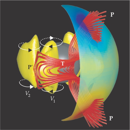
The geodynamo converts the kinetic energy of fluid motion in Earth’s core into magnetic energy. The motion of liquid iron couples to an initial, already existing magnetic field and drags the field lines in the direction of the flow via Faraday induction. (For a tutorial on how that works in a laboratory setting, see the article by Daniel Lathrop and Cary Forest, Physics Today, July 2011, page 40 .) This snapshot of the geodynamo in action illustrates the process in a planetary context.

The partially transparent outer spherical surface shown here represents the boundary between the electrically conducting, fluid outer core, where dynamo action is concentrated, and the solid mantle; the gray sphere represents the solid inner core. Earth’s rotation and the buoyant convection of molten metal produce vortices, depicted in yellow, that circulate the flow in directions set by the Coriolis force. Geomagnetic field lines are shown in red; blue shading on the core–mantle boundary denotes a negative, inwardly directed field, and yellow–red shading denotes a positive, outwardly directed field.

A feedback loop acts to sustain the illustration’s existing, south-pointing dipolar magnetic field P. As that field is sheared and twisted by the current in vortex V₁, two bundles, oriented east–west, of toroidal magnetic field T are induced, one on each side of the equator. Helical flow between vortices V₁ and V₂ then rotates and stretches the toroidal magnetic field bundles, which in turn induces a secondary south-pointing magnetic field P’. And that field tends to amplify the original dipolar field P. (Figure courtesy of Julien Aubert.)

References

1. P. Charbonneau, P. K. Smolarkiewicz, Science 340, 42 (2013). https://doi.org/10.1126/science.1235954
2. B. P. Weiss et al., Space Sci. Rev. 152, 341 (2010). https://doi.org/10.1007/s11214-009-9580-z
3. J. Arkani‐Hamed, J. Geophys. Res. 109, E03006 (2004). https://doi.org/10.1029/2003JE002195
4. T. Kleine et al., Nature 418, 952 (2002); https://doi.org/10.1038/nature00982
B. Wood, M. Walter, J. Wade, Nature 441, 825 (2006). https://doi.org/10.1038/nature047635. S. Labrosse, Phys. Earth Planet. Inter. 140, 127 (2003). https://doi.org/10.1016/j.pepi.2003.07.006
6. T. Lay, J. Hernlund, B. A. Buffett, Nat. Geosci. 1, 25 (2008). https://doi.org/10.1038/ngeo.2007.44
7. F. Nimmo, in Treatise on Geophysics, vol. 8, P. Olson, ed., Elsevier, Boston (2007), p. 31.
8. D. Bercovici, Y. Ricard, Phys. Earth Planet. Inter. 202, 27 (2012). https://doi.org/10.1016/j.pepi.2012.05.003
9. U. Christensen, J. Aubert, G. Hulot, Earth Planet. Sci. Lett. 296, 487 (2010). https://doi.org/10.1016/j.epsl.2010.06.009
10. P. Driscoll, P. Olson, Geophys. J. Int. 178, 1337 (2009). https://doi.org/10.1111/j.1365-246X.2009.04234.x
11. M. Pozzo et al., Nature 485, 355 (2012). https://doi.org/10.1038/nature11031
12. J. G. Ogg, in The Geologic Time Scale 2012, F. Gradstein et al., eds., Elsevier, Waltham, MA (2012), chap. 5.
13. J.-P. Valet, L. Meynadier, Y. Guyodo, Nature 435, 802 (2005). https://doi.org/10.1038/nature03674
14. C. L. Johnson, C. G. Constable, Geophys. J. Int. 122, 489 (1995). https://doi.org/10.1111/j.1365-246X.1995.tb07010.x
More about the authors
Peter Olson is a professor in the department of Earth and planetary sciences at Johns Hopkins University in Baltimore, Maryland.