Lagrangian coherent structures: The hidden skeleton of fluid flows

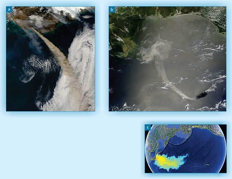
In April 2010, fine, airborne ash from a volcanic eruption in Iceland caused chaos throughout European airspace. The same month, the explosion at the Deepwater Horizon drilling rig in the Gulf of Mexico left a gushing oil well on the sea floor that caused the largest offshore oil spill in US history. A year later the Tohoku tsunami hit the coast of Japan, causing great loss of life, the Fukushima nuclear-reactor disaster, and the release of substantial amounts of debris and radioactive contamination into the Pacific Ocean.

Those three globally significant events, depicted in figure 1, share a common theme. In each case, material was released into the environment from what was essentially a point source, and predicting where that material would be transported by the surrounding oceanic or atmospheric flow was of paramount importance.

To predict the outcomes of such events, the standard approach is to run numerical simulations of the atmosphere or the sea and use the resulting velocity-field data sets to forecast pollutant trajectories. Although that approach does predict the future of individual fluid parcels, the predictions are highly sensitive to small changes in the time and location of release. Attempts to address the excessive sensitivity to initial conditions include running several different models for the same scenario. But that typically produces even larger distributions of advected particles—those transported by the fluid flow—and thus hides key organizing structures of that flow.

Furthermore, traditional trajectory analysis focuses on full trajectory histories that yield convoluted “spaghetti plots” that are hard to interpret. Improved understanding and forecasting therefore requires new concepts and methods that provide more insight into why fluid flows behave as they do.

Lagrangian coherent structures

Recently, ideas that lie at the interface between nonlinear dynamics—the mathematical discipline that underlies chaos theory—and fluid dynamics have given rise to the concept of Lagrangian coherent structures (LCSs), which provides a new way of understanding transport in complex fluid flows.

Although advances have been made in the detection of LCSs in fully three-dimensional flows, this article focuses primarily on the many advances that have been made for 2D flows. There, LCSs take the form of material lines—continuous, smooth curves of fluid elements advected by the flow. They are conceptually simpler than the 2D material surfaces required for LCSs in 3D flows. Furthermore, 2D flows are particularly relevant for studies of pollution transport on the ocean surface and on surfaces of constant density in the atmosphere.

Generally speaking, the LCS approach provides a means of identifying key material lines that organize fluid-flow transport. Such material lines account for the linear shape of the ash cloud in figure 1a, the structure of the oil spill in 1b, and the tendrils in the spread of radioactive contamination in 1c. More specifically, the LCS approach is based on the identification of material lines that play the dominant role in attracting and repelling neighboring fluid elements over a selected period of time. Those key lines are the LCSs of the fluid flow. To develop an understanding of them, we must first consider several ideas.

Lagrange versus Euler

There are two different perspectives one can take in describing fluid flow. The Eulerian point of view considers the properties of a flow field at each fixed point in space and time. The velocity field is a prime example of an Eulerian description. It gives the instantaneous velocity of fluid elements throughout the domain under consideration. The identity and provenance of fluid elements are not important; at any given point and instant, the velocity field simply refers to the motion of whatever fluid element happens to be passing.

By contrast, the Lagrangian perspective is concerned with the identity of individual fluid elements. It tracks the changing velocity of individual particles along their paths as they are advected by the flow. It’s the natural perspective to use when considering flow transport because patterns such as those in figure 1 arise from material advection.

Another driving force behind the development of the LCS approach is the concept of objectivity, or frame invariance. Characterizations of flow structures in terms of the properties of Eulerian fields such as the velocity field tend not to be objective; they don’t remain invariant under time-dependent rotations and translations of the reference frame. For instance, a common way to visualize flow fields is to use streamlines, which are Eulerian entities that follow the local direction of the velocity field at a given instant.

Traditionally, vortices in fluid flows have been identified as regions filled with closed streamlines. But velocity fields, and hence their streamlines, change when viewed from different reference frames. So what looks like a domain full of closed streamlines in one frame can appear completely different when viewed from another frame. For example, an unsteady vortex flow may look like a steady saddle-point flow in an appropriate rotating frame.

For unsteady flows, which are the rule rather than the exception in nature, there is no obvious preferred frame of reference. So any conclusion about transport-guiding dynamic structures should hold for any choice of reference frame. With regard to an oil spill, for example, interpretations of the organization of material transport cannot depend on whether the data are processed in the reference frame of an onshore radar observation station, a reconnaissance plane, or an orbiting satellite. Reliable forecasting of material transport calls for frame-invariant techniques.

Material lines

A detailed understanding of Lagrangian transport already exists for time-independent flows such as the steady saddle-point flow in figure 2a. Fluid parcels approaching a saddle point along a prominent line of flowing material that serves as a repulsive transport barrier (the so-called stable manifold) are ultimately drawn away from it toward an orthogonal material line that constitutes an attractive transport barrier (the unstable manifold) and carries them away from the saddle point. One manifold looks like the other with time reversed. The unstable manifold, despite its name, acts as a core organizing structure in the vicinity of the saddle point, attracting all nearby fluid particles, which then stretch out to adopt its shape.

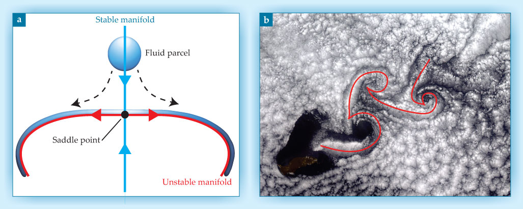
Prominent material lines are known to exist in periodic and quasiperiodic flows, where they serve as skeletons of observed tracer patterns. An example, shown in figure 2b, is suggested by the organized cloud features in the wake created by steady wind blowing past the Mexican island of Guadalupe. But finding them is rarely that easy. The identification of dynamical skeletons for material patterns in flows with complex spatial and temporal structure presents an ongoing challenge.

That’s because the mathematical methods used to identify key material lines in steady, periodic, and quasiperiodic flows rely on knowing the flow field for all time. But the flows that most need to be understood are typically aperiodic, and the associated velocity-field information is known only in the form of observational or numerical-simulation data sets for finite time intervals. As a result, even elementary concepts such as stable and unstable manifolds and saddle points are ill defined for aperiodic flows.

A modern characterization of repelling and attracting material lines has been emerging in fluid dynamics to facilitate the understanding of material transport by aperiodic, finite-time flows. The starting point is a 2D flow field,

dx/dt = u(x, t),

with position vector x = (x, y) and velocity vector u = (u, v) in the x, y plane.

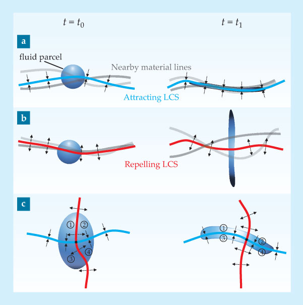
Assuming that the velocity field is observed for times t ranging over the finite interval [t₀, t₁], the LCSs of the flow during that interval are the material lines that repel or attract nearby fluid trajectories at the highest local rate relative to other material lines nearby. As shown in figure 3, the attraction and repulsion are orthogonal to the flow lines. Overall, the repelling and attracting LCSs play similar roles to the stable and unstable manifolds, respectively, of the saddle point in figure 2a. As illustrated in figure 3c, the repelling LCSs direct particles to different domains of the attracting LCSs.

A simple example

The relevance of the LCS approach to understanding fluid transport is nicely illustrated by the so-called double-gyre problem, ¹ presented in figure 4. Even though, as a time-periodic flow, it’s amenable to more traditional analysis, the double-gyre problem has become a canonical flow field for testing LCS ideas.

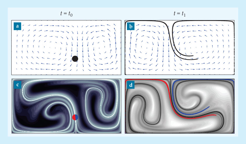
In figure 4, a circular blob of black dye is released at time t₀ in a flow comprising two oppositely swirling gyres (vortices) whose strengths and locations vary periodically in time. The arrows in figures 4a and 4b indicate the velocity field at t₀ and later at t₁.

By t₁, the dye has been stretched and transported throughout the fluid. But the new dye distribution is noticeably different from the shape of the velocity field at t₁. Much of it is stretched along the outer boundaries, and two dye streaks cut across to the right side of the domain. But there’s no dye drawn clockwise around the left vortex, even though that vortex is a strong feature of the velocity field.

Recall that if the flow were viewed from, say, a rotating reference frame, the form of the instantaneous velocity field would change significantly while the shape of the dye streak would remain the same. So the key question is, What frame-invariant structures are responsible for organizing the shape of the dye streak between t₀ and t₁?

Figure 4c presents a candidate LCS, the convoluted white line that cuts the initial dye patch into two parts, shown red and blue. That line is the strongest repelling structure at t₀. Bisecting the initial dye blob, it reveals that the blob is about to be separated by the flow field. Figure 4d reveals that by t₁, the two half-blobs have been drawn out along opposite sides of another candidate LCS (the black curve), the strongest attracting structure.

While the two LCS candidates are notably distinct from the features of the velocity fields, they clearly shape the transport of the dye blob. How does one find those LCSs?

The finite-time Lyapunov exponent

A pioneering insight into Lagrangian features in velocity-field data was provided 20 years ago by Raymond Pierrehumbert and Huijin Yang at the University of Chicago. ² They considered plots of the so-called finite-time Lyapunov-exponent (FTLE) field. The Lyapunov exponent is a measure of the sensitivity of a fluid particle’s future behavior to its initial position in the flow field.

To determine the FTLE field, one lets fluid particles flow under the action of the velocity field from t₀ and determines how much initially adjacent particles from a given location have separated by t₁. Regions of high separation have high FTLE values; they are locally the regions of most strongly diverging flow. Performing the same procedure in backward time, one identifies regions with high backward-time FTLE values. Those regions of strongest divergence in backward time are the regions of strongest local convergence in ordinary forward time.

In 2001 the complex patterns of FTLE distributions for physical flow fields were connected to LCSs by one of us (Haller), ³ who proposed that ridges of maxima in the FTLE field are, in fact, indicators of repelling LCSs in forward time and of attracting LCSs in backward time. The ridges were initially believed to be almost Lagrangian—that is, the flux of material across them was thought to be small. ¹

Two practical early examples of the FTLE approach were applications to pollution control off the coasts of Florida ⁴ and California. ⁵ In both cases, ocean-surface velocity fields, obtained over time from coastal high-frequency radar stations, were used to determine appropriate time windows for the necessary release of pollutants from coastal power stations. Since then, the FTLE approach has been applied to a great variety of problems such as blood flow in arteries, air traffic control, and flow separation by airfoils. ⁶

Equating LCSs with FTLE ridges provides an attractively simple computational tool. But it raises some fundamental mathematical questions that were initially overlooked. In particular, FTLE ridges can yield both false negatives and false positives in LCS detection. ⁷ Furthermore, the ridges are often far from being Lagrangian; the flux across them can be large.

Strainlines

To address the shortcomings of the FTLE approach for identifying LCSs, Haller and Mohammad Farazmand have now shown that repelling LCSs are, in fact, material lines whose initial positions are locally the most repelling strainlines for the time window in question. ⁸ As described in the box on page 46, strainlines are curves that are everywhere tangent to the eigenvector field of the Cauchy–Green strain tensor computed over the time window.

For 2D fluid flow, the Cauchy–Green tensor is a 2 × 2 symmetric, positive-definite matrix calculated for each initial position in the fluid. As such, it has positive eigenvalues (0 < λ₁ < λ₂), and its two eigenvectors (ξ₁ and ξ₂) are orthogonal. If the fluid is incompressible, λ₂ = 1/λ₁.

For 2D flows, the eigenvectors give the directions, in an infinitesimal sphere released at x₀, that will be mapped into the major and minor axes of the ellipsoid into which the sphere has formed at time t. The diameter of the initial sphere will be stretched and compressed by the ratio of the eigenvalues. By definition, strainlines are trajectories of the ξ₁ field. And the initial positions of LCSs are extracted as the locally strongest repelling or attracting strainlines. One gets later LCS positions by advecting the initial positions according to the flow map (see the box).

The LCSs thus obtained are truly Lagrangian entities with no material flux across them. They solve simple first-order, ordinary differential equations, and hence are smooth, parameterized curves. By contrast, extracting ridges from FTLE calculations has proven to be a challenging image-processing problem with no strict mathematical foundation.

The scenario from the Deepwater Horizon oil spill presented in figure 1b is a good example of the strainline approach. The satellite image, taken on 17 May 2010, reveals a large tendril of oil that extends southeast from the body of the main spill; that feature became known as the “tiger tail.” We have recently applied the strainline method of LCS detection to data from a numerical simulation of the Gulf of Mexico for that time period.

To expose the attracting LCSs responsible for shaping the tiger tail, we calculated the Cauchy–Green strain tensor for the backward-time window from 17 May to 14 May. From that information, the ξ₁ and ξ₂ vector fields were determined and are presented in figure 5a. In general, any point in the domain is a starting point of a strainline—that is, a trajectory of the ξ₁ field.

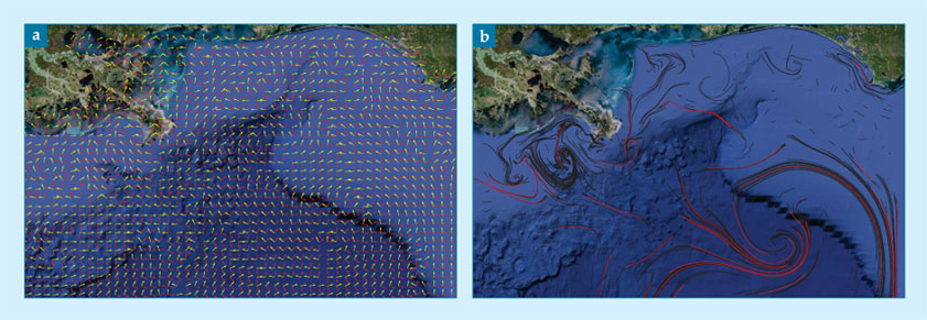
Several such strainlines are marked in figure 5b. The strongest attracting strainlines (those with the largest averaged values of λ₂) are highlighted in red as the LCSs responsible for shaping the tiger tail. The same procedure can be carried out in forward time (from 14 May to 17 May) to identify the repelling structures that played a key role in disrupting the original shape of the oil spill.

LCS-based decision making

The results shown in figure 5, revealing the attracting LCSs responsible for shaping the Gulf oil spill between 14 May and 17 May, can be called a “hindcast.” They provide an explanation of something that happened, based on data gathered beforehand. Nonetheless, the analysis yields valuable insight because it provides a framework for explaining why things behaved as they did. Building on that newfound knowledge, however, one must ask whether LCS methods can help forecast features such as the tiger tail.

A first step toward forecasting is called “nowcasting,” the accurate determination of the present state of the system from available information. The ability to nowcast LCSs means that the current location of key transport barriers in the ocean or atmosphere would be known, which in itself would be a significant achievement. To accomplish that, the way forward is to use the ever more comprehensive, reliable, and up-to-the-minute data available through satellite measurements and local monitoring stations (for example, high-frequency radar and ocean drifters) in combination with large-scale numerical simulations.

Returning to the Deepwater Horizon spill as a demonstration of the benefits of accurate nowcasting, a recent analysis ⁹ has revealed that a single LCS pushed the oil spill toward the coast of Florida for about two weeks in June 2010, as shown in figure 6a. Had that information been available at the time, it would likely have lent greater confidence to decision-making strategies for the Gulf Coast.

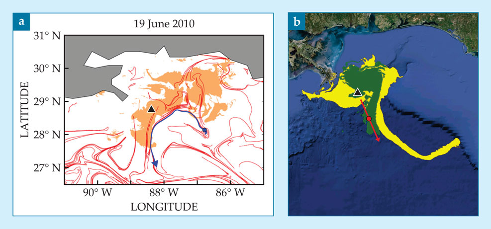
The logical extension of nowcasting is the anticipation that as the accuracy of numerical simulations improves, the velocity-field data they generate can support increasingly reliable LCS predictions. More significant, however, is the discovery that so-called hyperbolic cores of LCSs can be used to forecast strong events such as the tiger tail from nothing but information obtained up to the present ⁹ (see figure 6b).

A hyperbolic core of an attracting LCS is a short segment of the LCS that has uniformly strong attraction—that is, where λ₂ throughout the segment is within the top 1% for the whole domain. If the flow behaves in a reasonably 2D manner, then volume conservation requires a strongly repelling LCS to stretch significantly. Thus the region behaves like a saddle point. The identification of a hyperbolic core provides predictive capability because it indicates a developing transport event, like the tiger tail, that’s too strong to be halted by short-term future events.

Outlook

Yielding profound insight about transport in complex, time-dependent flows, the study of LCSs is now a vibrant research field. Applications abound. In the coming years, the LCS approach may well prove to be crucial, for example, in the planned response to the large quantity of debris from the Tohoku tsunami that is approaching the US West Coast. In the longer term, LCS methods are expected to yield improved pollution monitoring and search-and-rescue strategies along seacoasts. Ultimately, LCS applications should also improve our understanding of transport in industrial and biological flows.

Although the mathematical theory of attracting and repelling LCSs is now well established, important practical challenges remain, such as acquisition of the requisite velocity data. For coastal regions, the presence of high-frequency radar stations that can provide the necessary data is becoming increasingly common. And the fast numerical processing of such data sets is now within reach, given the broad availability of parallel-computing platforms.

A recent advance in LCS theory provides a general extraction tool for all key Lagrangian structures in unsteady flows. Such structures include attracting and repelling LCSs as well as coherent vortex-type patterns (called elliptic LCSs) and jet-type patterns (called shear LCSs). Via that approach, LCSs can be unmasked by their telltale property of stretching less than neighboring material lines do. ¹⁰

A challenging computational task will be to follow the evolution of LCSs as they are advected in forward or backward time by the fluid flow. That’s more than simply locating a repelling or attracting LCS, respectively, at the beginning or end of a time window. It requires the development of effective numerical approaches to the advection of strongly unstable material lines.

It also remains to connect LCS analysis to other recent approaches to Lagrangian coherence such as the set-theoretical approach of Michael Allshouse and Jean-Luc Thiffeault ¹¹ and the probabilistic methods of Gary Froyland and Katherine Padberg. ¹²

The development of rigorous and efficient LCS methods for 3D flows is under way. Such methods will reveal the key 2D material surfaces that act as transport barriers in 3D. That will yield better understanding of flow transport in a great variety of physical systems.

References

1. S. C. Shadden, F. Lekien, J. E. Marsden, Physica D 212, 271 (2005). https://doi.org/10.1016/j.physd.2005.10.007
2. R. T. Pierrehumbert, H. Yang, J. Atmos. Sci. 50, 2462 (1993). https://doi.org/10.1175/1520-0469(1993)050<2462:GCMOIS>2.0.CO;2
3. G. Haller, Physica D 149, 248 (2001). https://doi.org/10.1016/S0167-2789(00)00199-8
4. F. Lekien et al., Physica D 210, 1 (2005). https://doi.org/10.1016/j.physd.2005.06.023
5. C. Coulliette et al., Environ. Sci. Technol. 41, 6562 (2007). https://doi.org/10.1021/es0630691
6. T. Peacock, J. Dabiri, Chaos 20, 017501 (2010). https://doi.org/10.1063/1.3278173
7. G. Haller, Physica D 240, 574 (2011). https://doi.org/10.1016/j.physd.2010.11.010
8. M. Farazmand, G. Haller, Chaos 22, 013128 (2012). https://doi.org/10.1063/1.3690153
9. M. J. Olascoaga, G. Haller, Proc. Natl. Acad. Sci. USA 109, 4738 (2012). https://doi.org/10.1073/pnas.1118574109
10. G. Haller, F. J. Beron-Vera, Physica D 241, 1680 (2012). https://doi.org/10.1016/j.physd.2012.06.012
11. M. R. Allshouse, J.-L. Thiffeault, Physica D 241, 95 (2012). https://doi.org/10.1016/j.physd.2011.10.002
12. G. Froyland, K. Padberg, Physica D 238, 1507 (2009). https://doi.org/10.1016/j.physd.2009.03.002
More about the authors
Thomas Peacock is a professor of mechanical engineering at the Massachusetts Institute of Technology in Cambridge. George Haller is a professor of nonlinear dynamics at ETH Zürich in Switzerland.