Imaging with ambient noise
DOI: 10.1063/1.3490500
Recent developments in seismology, ultrasonics, and underwater acoustics have led to a radical change in the way scientists think about ambient noise—the diffuse waves generated by pressure fluctuations in the atmosphere, the scattering of water waves in the ocean, and any number of other sources that pervade our world. Because diffuse waves consist of the superposition of waves propagating in all directions, they appear to be chaotic and random. That appearance notwithstanding, diffuse waves carry information about the medium through which they propagate.
During the past decade, experimental and theoretical work has shown that such waves can produce an elastic response to a point source in the medium. That response is valuable because it can be used to determine the properties of the medium—for instance, using waves reflected from the medium’s discontinuities to provide the location and nature of those discontinuities or waves transmitted through the medium to infer their acoustic or seismic velocity. Perhaps surprisingly, the elastic response can be determined from recorded diffuse waves through a simple processing step: cross-correlation, a statistical measure of the waveforms’ similarities at different points in space as a function of the time lag applied to one of them.
More specifically, if one were to measure a diffuse wave field that propagates through two arbitrary points in space, the cross-correlation of the two noise registrations would give the same response of the medium that would be measured if there were a source at one of the two points and a receiver at the other. Thus, by just listening passively to ambient noise and applying a simple data-processing operation, one obtains the same information that would be obtained in a controlled experiment using an impulsive source such as an explosion or earthquake to generate a pressure field. In the case of ambient noise, however, one speaks of a virtual source, not a real source.
Retrieving the Green function
Imagine a closed system that vibrates in response to random noise sources. Given a set of normal modes un (x), the Green function that describes the impulsive response can be written
where H(t) is the Heaviside function, zero for negative time and 1 for positive time, and ω n is the angular frequency of mode n.
We outline Oleg Lobkis and Richard Weaver’s derivation of such a Green function, 6 starting with a state of motion in which the time derivative of pressure fluctuations is given by
where the modal coefficients an and bn are random numbers with zero mean. The modes are assumed to be excited with equal energy and have uncorrelated excitations. That is,
where 〈 〉 denotes the expectation value and S is the modes’ excitation energy.
Next, consider the time-averaged cross-correlation of the field at two locations x A and x B,
The length of the time integration is denoted by T, and τ denotes the lag time used in the correlation. Inserting the normal-mode expansion (2) in that integral gives a double sum over modes. After taking the expectation value, the double sum reduces to the following single sum by virtue of the expectation values of equation (3):
A comparison of this equation with the general Green function (1) shows that when τ > 0, the last term is equal to SG(x a,x b,τ), and when τ < 0, it is equal to SG(x a,x b,−τ). Hence,
The expectation value of the cross-correlation thus gives the superposition of the Green function and its time-reversed counterpart.
That principle holds no matter how complex the heterogeneities and boundaries of the medium. What’s more, there are numerous cases in which it can be advantageous to use a virtual source. For example, although seismologists routinely use waves excited by earthquakes to image Earth’s deep structure, the earthquakes themselves occur only in certain regions of the planet, which restricts how well seismic waves illuminate faraway parts of the subsurface. But in the case of ambient noise, every seismometer can act as a source. Indeed, by deploying dense networks of seismometers, researchers have reconstructed with unprecedented detail the structure and properties of Earth’s crust in many parts of the world. 1
Examples go well beyond seismology. For instance, researchers have used the noise of thermal fluctuations in an aluminum specimen as the basis for ultrasonic pulse-echo measurements of its structure; 2 extracted coherent wave-fronts from acoustic noise in the ocean and atmosphere 3 (data that, in the case of the ocean, yield the speed of sound and thus constrain its temperature and salinity); and measured the stiffness of muscle tissue by monitoring the mechanical vibrations that occur during the muscle’s contractions. 4 Moreover, the use of ambient noise is especially convenient in cases where it’s not practical or even safe to place a real noise source, such as in a crowded urban environment or in the ocean near sensitive marine mammals.
Because the response to an impulsive point source is, by definition, equal to a Green function, the methodology of turning noise into a signal is often called Green function retrieval or, in seismological applications, seismic interferometry, a term introduced by the University of Utah’s Gerard Schuster. 5 “Interferometry” is, in that context, borrowed from radio astronomy, in which it refers to cross-correlation methods applied to radio signals from distant objects.
Closed and open systems
In their early work in 2001 extracting the Green function from ultrasonic noise correlations in aluminum, University of Illinois physicists Oleg Lobkis and Richard Weaver provided a beautiful derivation of the method by assuming that all normal modes in the material are excited by uncorrelated noise sources of equal strength, as outlined in the
Lobkis and Weaver’s elegant normal-mode formulation came from their analysis of a closed system—a block of aluminum. Although Earth is also a finite body with a free surface, it’s often more natural to consider it an open system. After all, the penetration depth of the waves in many seismic observations is far less than Earth’s diameter, so the waves never sample the entire planet. Fortunately, for those circumstances, the data-processing technique suggested by Lobkis and Weaver is still valid, although the theoretical justification is different. One can, in fact, relate the principle of Green function retrieval to time reversal, as described by articles in Physics Today by Mathias Fink (March 1997, page 34 ) and by Carène Larmat, Robert Guyer, and Paul Johnson (August 2010, page 31 ).
The analysis of industrial noise propagating down a monitoring well at a Canadian heavy-oil production facility, as illustrated in figure 1(a), provides an example of Green function retrieval in the simplest situation, in which wave propagation is essentially one dimensional. In 2008 Masatoshi Miyazawa and colleagues took field data of the ground motion excited by the pumps and other industrial machinery used to inject steam into numerous wells in order to melt the heavy oil.
8
The noise propagates down an array of geophones in the monitoring well from the shallowest geophone (A) to the deepest (B). Although the two signals in figure

Figure 1. (a) At an oil-production facility in Canada, a layer of heavy oil (pink) is liquefied by the injection of steam through a series of underground wells (gray), as depicted in the schematic. Noise (red star) from industrial pumps and other equipment is generated at the surface and recorded along a vertical array of geophones (blue dots). (b) As the noise signal propagates down the array, geophones A and B record the wave motion at the shallowest and deepest sites. (c) Each of the eight traces is the result of cross-correlating one day of noise recorded by geophone B with noise recorded by another geophone in the series. The projection of the red line along the time axis gives the travel time of a compressive wave propagating from A to B.
(Adapted from
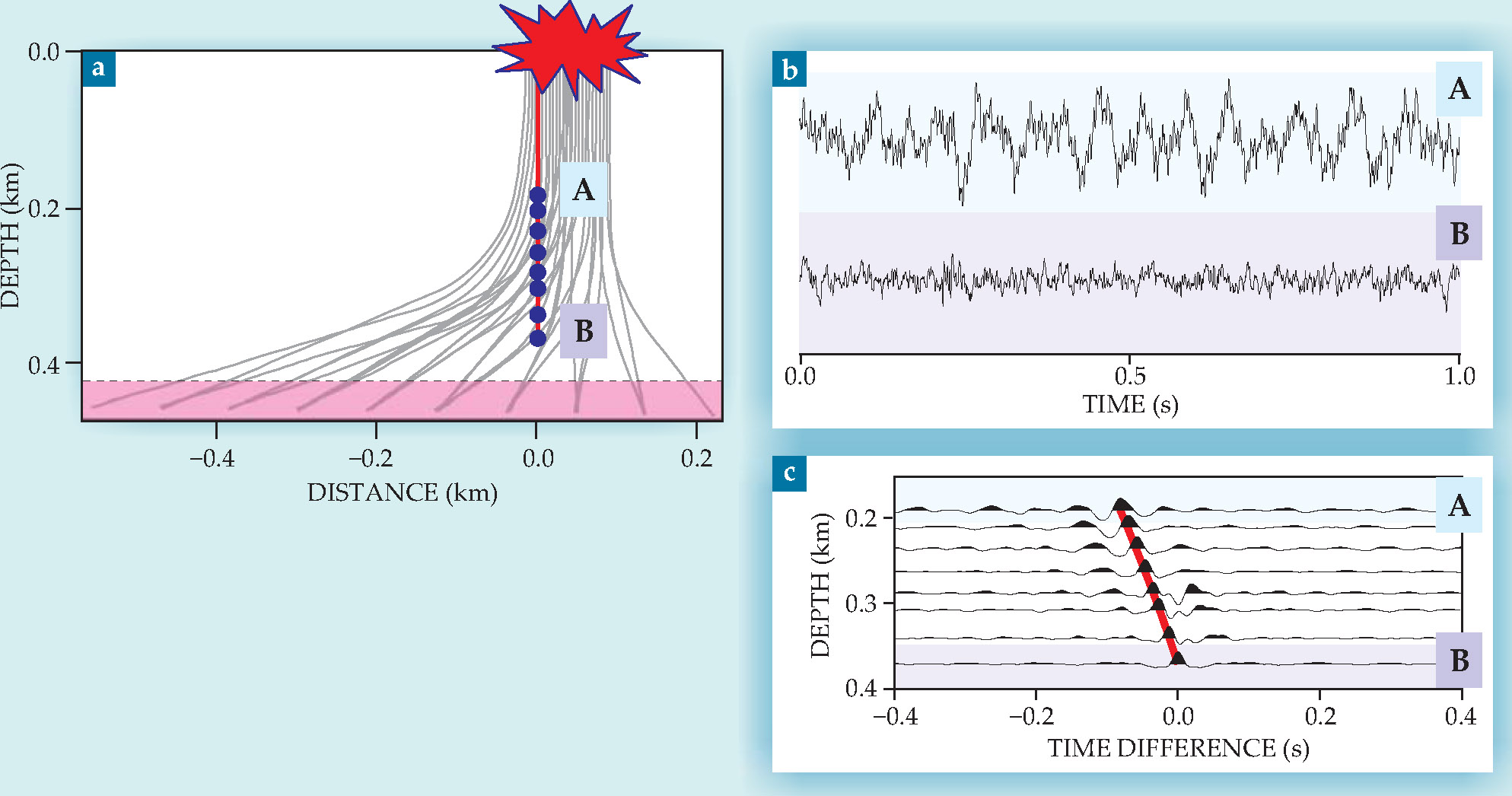
a time-averaged integral in which ν represents the waveform at the two geophones, τ represents the time lag of a wave’s arrival at B after passing A, and T represents the integration time—about 15 s in this example. The ensemble average is then estimated by averaging the result over all 15-s intervals in one day. After bandpass filtering, the results of processing noise recorded at B with that of all the other sensors give the eight traces shown in figure
The cross-correlation process reveals a pulse that propagates down the array and is visible as the downward-propagating wave. The red line gives the travel time of that wave computed from known properties of the rock. And the wave itself can be parsed into compressive- and shear-wave components by cross-correlating the vertical and horizontal components of the noise recorded at each geophone. By repeating the cross-correlation for two perpendicular horizontal components Miyazawa and colleagues retrieved the Green function for two downward-propagating shear waves with perpendicular polarizations. The tiny differences in travel time between those shear waves provide information on the orientation of cracks in the rock and hence the directional permeability of the rock to the flow of fluid.
The cross-correlation of two signals depends, by definition, on the time difference of those signals. Suppose that the travel time of a noise burst from the source to receiver B is given by t B = (z B − z S)/c, where z B is the depth of geophone B, z S is the depth of the noise source, and c is the wave velocity. The noise burst arrives at geophone A at time t A = (z A − z S)/c. Cross-correlation of the noise bursts at sensors A and B extracts an impulsive wave arriving at time tA − tB =-(zB − zA)/c. Note that the time is independent of the source depth z S, thanks to the fact that the waves propagating from the source to sensors A and B share a common path.
Since z B > z A, the cross-correlation yields an arrival time t A − t B < 0. And indeed, the waves in figure
The physical reason for retrieving that superposition is that in a truly diffusive field, waves propagate with equal strength from x A to x B as they do in the opposite direction. The Green function, moreover, is causal, which means that G(x A,x B,t) is only nonzero for t > 0 and G(x A,x B,-t) is only nonzero for t < 0. Separating the two contributions to the cross-correlation can be achieved by parsing the retrieved signal for t > 0 and t < 0, respectively.
Toward higher dimensions
The simplicity of the field example in figure

Figure 2. Green function retrieval in a two-dimensional open system. (a) Point sources of noise (red dots) whose positions are denoted by radius r S and azimuth φS send waves to receivers at x A and x B. The dashed lines delimit zones in which the cross-correlation of noise recorded at receivers A and B does not, to first order, depend on the angle φS. (b) The cross-correlation of signals that arrive at A and B from each source is plotted as a function of the lag time of the cross-correlation and source azimuth φS. The dashed lines delimit zones where waves constructively interfere. (c) The sum of the correlations in the plot yields two waves at +0.6 s that propagate between the receivers in opposite directions and are described by the Green function and its time-reversed counterpart G (x A,x B,t) + G (x A,x B,-t).
(Adapted from K. Wapenaar, J. Fokkema, R. Snieder,
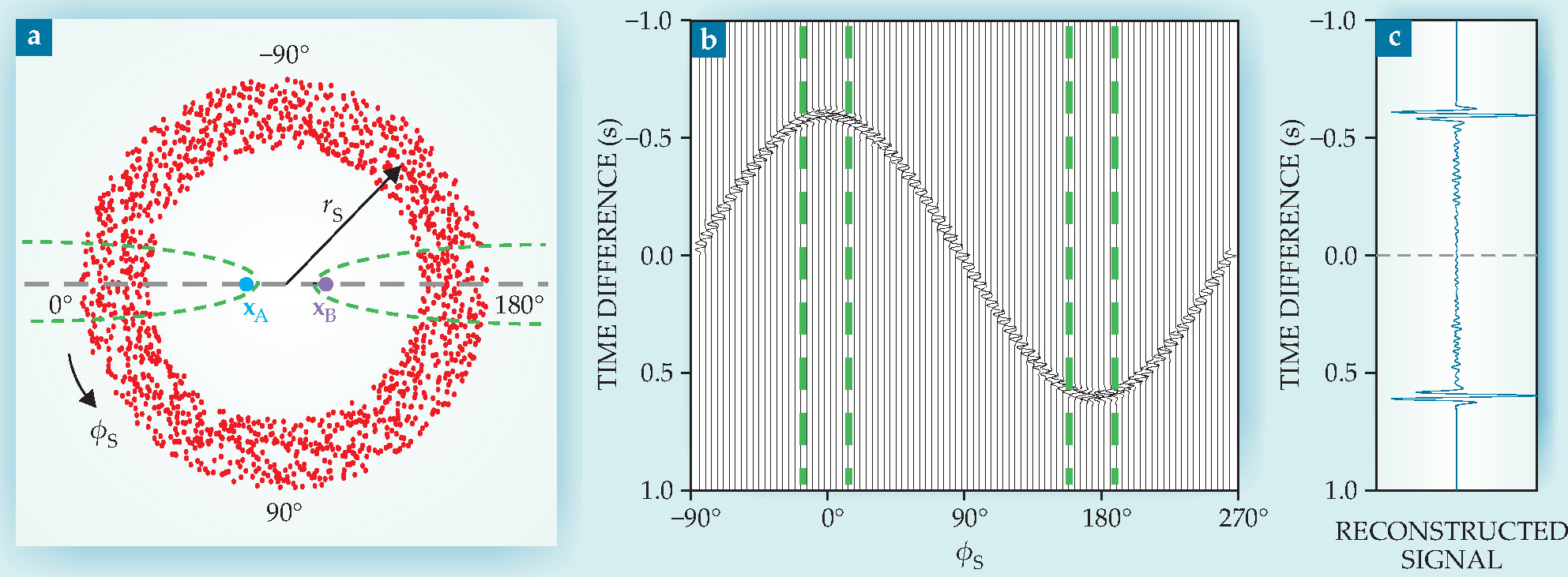
That 2D example consists of many point sources, denoted by red dots, distributed over a “pineapple slice,” each emitting transient signals that propagate at 2000 m/s through a homogeneous medium to two receivers at x A and x B, 1200 m apart. The positions of those sources in figure
A source in figure
In the sum, only signals arriving at +0.6 s survive. Waves emitted by sources in the vicinity of φS = 0° and φS = 180° —the so-called stationary-phase zones delimited by green dashed lines in figures
The noise that exists between the two events in figure
Tomography
One of the most widely used applications of ambient-noise interferometry is the retrieval of seismic surface waves between seismometers, first demonstrated in 2003 by Michel Campillo and Anne Paul at Joseph Fourier University, 11 and the subsequent tomographic determination of the waves’ velocity distribution in Earth’s crust and mantle. 1 In layered media, surface waves consist of several propagating modes, of which the fundamental mode is usually the strongest. As long as only the fundamental mode is considered, surface waves can be seen as an approximate solution of a 2D scalar wave equation with a frequency-dependent propagation velocity. By analogy with the analysis of figure 2, the Green function of the fundamental mode of a surface wave can thus be extracted by cross-correlating ambient-noise recordings from any two seismometers. Indeed, when many seismometers are available, the correlation can be repeated for any combination of two seismometers. Each seismometer becomes a virtual source, the response to which is observed by all other seismometers.
Earth’s surface waves come in two types: Rayleigh waves, which are polarized in the vertical plane in the direction of propagation, and Love waves, which are polarized horizontally, perpendicular to the direction of propagation. Figure 3, from work by Fan-Chi Lin of the University of Colorado at Boulder and his colleagues, shows a beautiful example of the Rayleigh-wave response to a virtual source southeast of Lake Tahoe, California. 12 The white triangles surrounding the virtual source (the white star) represent the more than 400 seismometers that make up Earthscope’s US-Array, spread throughout the western US.

Figure 3. A large array of seismometers (white triangles) in the western US captures the seismic response of a virtual source (white star), located just southeast of Lake Tahoe, California, at a moment in time. The snapshot, taken 200 s after a virtual impulse, was obtained by cross-correlating three years of ocean-generated ambient noise recorded at the station denoted by the star with noise recorded at each of the other stations. The result is a surface wave that propagates from the virtual source outward through the other stations in the array. The approach offers an unprecedented illumination of Earth’s crust.
(Adapted from
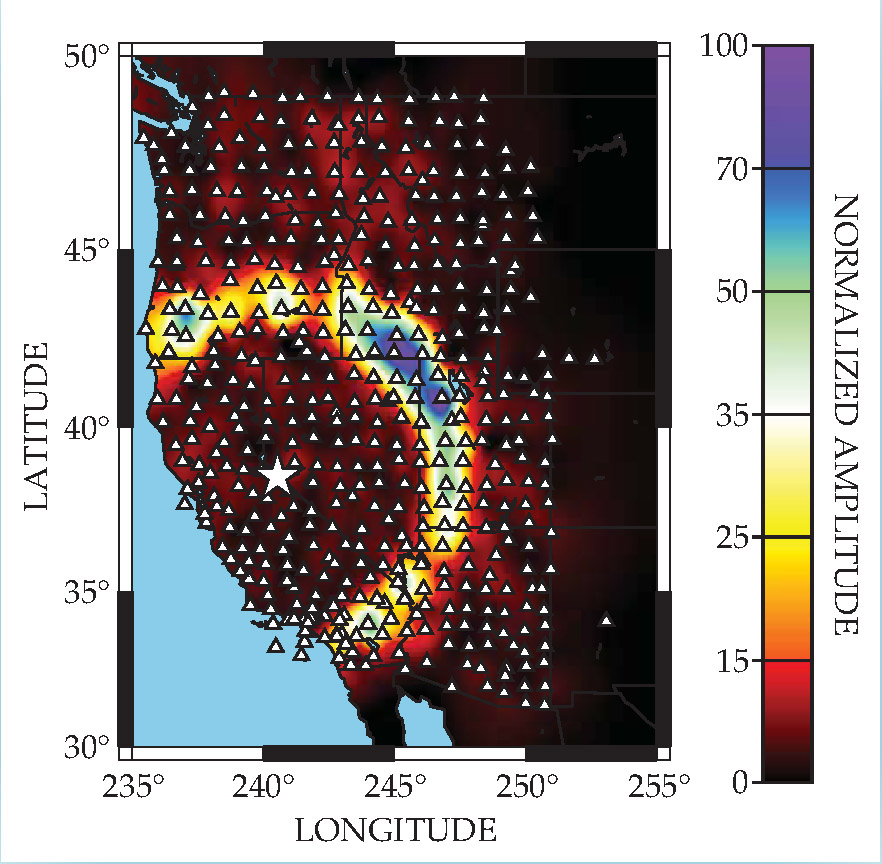
Ocean-generated ambient noise was recorded by the US-Array between October 2004 and November 2007. The interference of ocean waves propagating in opposite directions produces pressure fluctuations at the ocean bottom that excite seismic waves in solid Earth. Since the seismic noise comes from the ocean, it is far from isotropic. That means that the correlation of noise between any two stations does not yield time-symmetric results like those in figure 2. However, as long as one of the stationary-phase zones is sufficiently covered with sources, it is possible to retrieve either G(x A,x B,t) or G(x A,x B,-t).
Lin and colleagues captured the snapshot shown in figure 3 by cross-correlating, one by one, the noise recorded at one station (the white star) with that recorded at each of the others. The amplitudes exhibit azimuthal variation due to the anisotropic illumination by the ambient noise. The response can be used for tomographic reconstruction of the Rayleigh-wave velocity in the crust and the directional dependence of that velocity. The Rayleigh-wave velocity in turn can be used to infer the temperature and composition of the crust, and the directional dependence helps constrain the tectonic deformation the region has experienced.
Florent Brenguier of the Institut de Physique du Globe de Paris and colleagues have extended that approach to 3D tomographic inversion. 13 From noise measurements at the Piton de la Fournaise volcano they retrieved the Rayleigh-wave group velocity distribution as a function of frequency and used it to derive a 3D shear-wave velocity model of the volcano’s interior. In the past couple of years, such applications of direct surface-wave interferometry have expanded spectacularly. Their success is largely explained by the fact that surface waves are by far the strongest waves excited by ambient seismic noise.
The reflection response
So far, we have considered waves that propagate as transmitted waves between receivers. Let’s next consider the important case of reflected waves, which form the basis for delineating discontinuities in, for example, Earth or the human body. As early as 1968, Stanford University geophysicist Jon Claerbout showed that for a horizontally layered medium, the autocorrelation of a transmission response gives its reflection response. 14 That means that if one has measured the waves that are transmitted through a layered medium, one can infer the waves that are reflected within it.
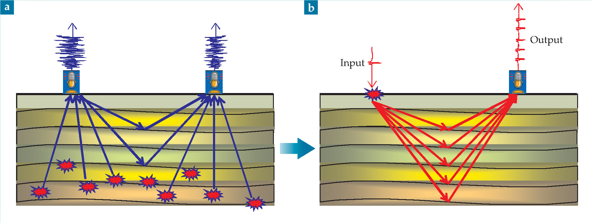
To appreciate how that works in arbitrary inhomogeneous media, consider the situation in figure 4(a), where noise sources—for example, from micro-earthquakes or far-off events whose waves refract upward—illuminate a stack of reflecting layers from below. Noise sources launch waves that propagate to one of the receivers, reflect off the free surface, then reflect again from layers in Earth before propagating to the other receiver. Cross-correlation of the waves recorded at two receivers gives the reflected waves that propagate between them, as shown in figure

Figure 4. Retrieving the reflection response from ambient noise. (a) Consider an arbitrary, inhomogeneous, lossless medium with noise sources (red) buried in its subsurface and two geophones at its free surface. Those noise sources send waves that reach the geophones directly or after reflecting from subsurface discontinuities. (b) The cross-correlation of noise signals recorded by the two geophones reveals the same reflection response that would be observed by one of the geophones if there were an impulsive source at the position of the other.
Deyan Draganov from Delft University of Technology and colleagues applied that methodology to ambient noise recorded by Shell in a desert area near Ajdābiyah, Libya. 15 Eleven hours of noise were recorded along eight parallel geophone lines extending about 20 km and separated by 500 m. Each line consisted of approximately 400 groups of geophones evenly spaced. Much of the processing was dedicated to suppressing surface waves caused by nearby road traffic. The cross-correlation approach retrieved the reflection responses of many virtual sources at the surface. Those responses were then turned into a 3D image of the subsurface using standard seismic imaging methods. Cross sections are shown in figure 5. The horizontal stripes correspond to discontinuities in Earth associated with the juxtaposition of different rock types.

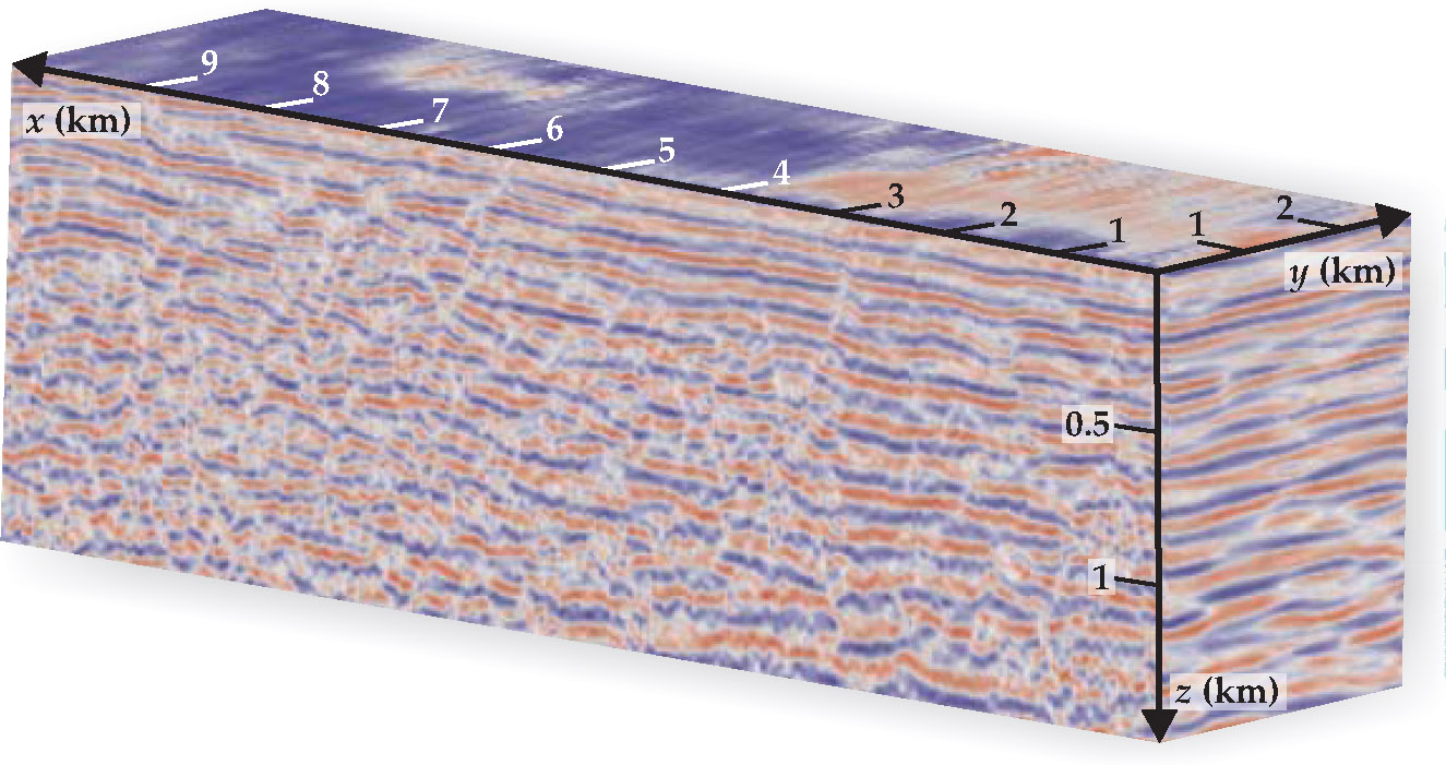
Figure 5. A three-dimensional reflection image of the geology beneath the Libyan desert, based on data obtained by cross-correlating 11 hours of ambient noise. The horizontal stripes indicate discontinuities in Earth’s crust due to the juxtaposition of different rock types. Such images are essential for the exploration and production of oil and gas.
(Adapted from
Such images help seismologists understand the geologic structure of the subsurface and are a major tool in the exploration and production of oil and gas. Potential applications of the method range from exploration for hydrocarbons in environmentally sensitive areas, where active sources cannot be used, to the crustal- and even global-scale imaging of Earth’s substructure.
Further applications
Researchers are not limited to ambient seismic noise on Earth for their geophysical explorations. Observations of ambient noise on the surfaces of the Sun and the Moon have been used to retrieve helioseismological shot records and the time-dependent impulse response of the Moon. 16 Developments are now under way to retrieve Earth’s electromagnetic impulse response from natural and manmade variations in its electromagnetic fields. Cross-correlating seismic noise with electromagnetic noise observations may yield the electro-seismic response and thus provide a basis for imaging the poroelastic properties of the subsurface. The theory for Green function retrieval from noise has been generalized for a wide class of linear equations, which means the method is applicable to noise correlations in wave fields ranging from those governed by quantum mechanics to those typically encountered in structures such as buildings and bridges. 17
When noise sources persist for long times, a system’s Green function can be extracted on a quasi-continuous basis. That makes the method particularly useful for passive monitoring. Applications include detecting changes in seismic velocity due to the relaxation in stress after an earthquake and monitoring damage in metal structures. 18
More broadly, the wave motion in Earth depends on both the properties of Earth and the mechanism of the seismic source. In the traditional seismic method, that source must be known if the recorded waves are to be used to infer the structure of Earth’s crust or mantle. When the impulse response is retrieved from noise measurements, the mechanism of the source—a virtual source—is known, which eliminates one unknown.
The fact that Green function retrieval by cross-correlation leads to new responses from measured field fluctuations has generated much enthusiasm this past decade and prompted collaborations among researchers in seismology, acoustics, and electromagnetic prospecting.
A major advantage of statistical correlations is that they require no knowledge either of the medium’s parameters or of the positions or timing of the actual noise sources. The processing is driven entirely by noise signals that pass through different points in space and time. Thanks partly to that simplicity—and the ubiquity of ambient noise sources around us—we expect many new applications to emerge in the coming years.
References
1. N. M. Shapiro et al., Science 307, 1615 (2005); https://doi.org/10.1126/science.1108339
K. G. Sabra et al., Geophys. Res. Lett. 32, L14311 (2005), https://doi.org/10.1029/2005GL023155 .2. R. L. Weaver, O. I. Lobkis, Phys. Rev. Lett. 87, 134301 (2001). https://doi.org/10.1103/PhysRevLett.87.134301
3. P. Roux et al., J. Acoust. Soc. Am. 116, 1995 (2004); https://doi.org/10.1121/1.1797754
M. M. Haney, Geophys. Res. Lett. 36, L19808 (2009), https://doi.org/10.1029/2009GL040179 .4. K. G. Sabra et al., Appl. Phys. Lett. 90, 194101 (2007). https://doi.org/10.1063/1.2737358
5. G. Schuster, Seismic Interferometry, Cambridge U. Press, New York (2009).
6. O. I. Lobkis, R. L. Weaver, J. Acoust. Soc. Am. 110, 3011 (2001). https://doi.org/10.1121/1.1417528
7. H. B. Callen, T. A. Welton, Phys. Rev. 83, 34 (1951); https://doi.org/10.1103/PhysRev.83.34
J. Weber, Phys. Rev. 101, 1620 (1956). https://doi.org/10.1103/PhysRev.101.16208. M. Miyazawa, R. Snieder, A. Venkataraman, Geophysics 73(4), D35 (2008). https://doi.org/10.1190/1.2937172
9. R. Snieder, Phys. Rev. E 69, 046610 (2004); https://doi.org/10.1103/PhysRevE.69.046610
R. Snieder, K. Wapenaar, K. Larner, Geophysics 71(4), SI111 (2006). https://doi.org/10.1190/1.221150710. K. Mehta et al., Leading Edge 27, 620 (2008); https://doi.org/10.1190/1.2919580
Y. Fan, R. Snieder, Geophys. J. Int. 179, 1232 (2009). https://doi.org/10.1111/j.1365-246X.2009.04358.x11. M. Campillo, A. Paul, Science 299, 547 (2003). https://doi.org/10.1126/science.1078551
12. F. -C. Lin, M. H. Ritzwoller, R. Snieder, Geophys. J. Int. 177, 1091 (2009). https://doi.org/10.1111/j.1365-246X.2009.04105.x
13. F. Brenguier et al., Geophys. Res. Lett. 34, L02305 (2007), https://doi.org/10.1029/2006GL028586 .
14. J. F. Claerbout, Geophysics 33, 264 (1968); https://doi.org/10.1190/1.1439927
for a generalization to arbitrary, inhomogeneous media, see K. Wapenaar, Phys. Rev. Lett. 93, 254301 (2004). https://doi.org/10.1103/PhysRevLett.93.25430115. D. Draganov et al., Geophysics 74(5), A63 (2009). https://doi.org/10.1190/1.3193529
16. J. Rickett, J. Claerbout, Leading Edge 18, 957 (1999); https://doi.org/10.1190/1.1438420
E. Larose et al., Geophys. Res. Lett. 32, L16201 (2005), https://doi.org/10.1029/2005GL023518 .17. R. Snieder, K. Wapenaar, U. Wegler, Phys. Rev. E 75, 036103 (2007); https://doi.org/10.1103/PhysRevE.75.036103
R. Weaver, Wave Motion 45, 596 (2008). https://doi.org/10.1016/j.wavemoti.2007.07.00718. U. Wegler, C. Sens-Schönfelder, Geophys. J. Int. 168, 1029 (2007); https://doi.org/10.1111/j.1365-246X.2006.03284.x
F. Brenguier et al., Science 321, 1478 (2008); https://doi.org/10.1126/science.1160943
A. Duroux et al., J. Acoust. Soc. Am. 127, 3311 (2010). https://doi.org/10.1121/1.3397447
More about the authors
Roel Snieder is the W. M. Keck Distinguished Professor of Basic Exploration Science and director of the Center for Wave Phenomena at the Colorado School of Mines in Golden. Kees Wapenaar is a professor of applied geophysics at Delft University of Technology in Delft, the Netherlands.
Roel Snieder, 1 Colorado School of Mines, Golden, US .
Kees Wapenaar, 2 Delft University of Technology, Delft, Netherlands .


