Data analysis: Frequently Bayesian

All experiments have uncertain or random aspects, and quantifying randomness is what probability is all about. The mathematical axioms of probability provide rules for manipulating the numbers, and yet pinning down exactly what a probability means can be difficult. Attempts at clarification have resulted in two main schools of statistical inference, frequentist and Bayesian, and years of raging debate.

A role for subjectivity?

For frequentists, a probability is something associated with the outcome of an observation that is at least in principle repeatable, such as the number of nuclei that decay in a certain time. After many repetitions of a measurement under the same conditions, the fraction of times one sees a certain outcome—for example, 5 decays in a minute—tends toward a fixed value.

The idea of probability as a limiting frequency is perhaps the most widely used interpretation encountered in a physics lab, but it is not really what people mean when they say, “What is the probability that the Higgs boson exists?” Viewed as a limiting frequency, the answer is either 0% or 100%, though one may not know which. Nevertheless, one can answer with a subjective probability, a numerical measure of an individual’s state of knowledge, and in that sense a value of 50% can be a perfectly reasonable response. The term “degree of belief” is used in the field to describe that subjective measure.

Both the frequentist and subjective interpretations provoke some criticism. How can scientists repeat an experiment an infinite number of times under identical conditions, and would the empirical frequency be anything that a mathematician would recognize as a mathematical limit? On the other hand, it surely seems suspect to inject subjective judgments into an experimental investigation. Shouldn’t scientists analyze their results as objectively as possible and without prejudice?

Regardless of interpretation, any probability must obey an important theorem published by Thomas Bayes in 1763. Suppose A and B represent two things to which probabilities are to be assigned. They may be outcomes of a repeatable observation or perhaps hypotheses to be ascribed a degree of belief. As long as the probability of B, P(B), is nonzero, the conditional probability of A given B, P(A|B), may be defined as P(A|B) = P(A and B)/P(B).

Here P(A and B) means the probability that both A and B are true. Consider, for example, rolling a die. A could mean “the outcome is even” and B “the outcome is less than 3.” Then “A and B” is satisfied only with a roll of two. The imposed condition, B, says that the spacscodee of possible outcomes is to be regarded as some subset of those initially specified. As a special case, B could be the initially specified set; in that sense all probabilities are conditional.

Now A and B are arbitrary labels; so as long as P(A) is nonzero, one can reverse the labels A and B in the equation defining P(A|B) to obtain P(B|A) = P(B and A)/P(A). But the stipulation “A and B” is exactly the same as “B and A,” so their probabilities must also be equal. Therefore, one can solve the respective conditional-probability equations for P(A and B) and P(B and A), set them equal, and arrive at Bayes’s theorem,

$$\text{P}\left(\text{A}\mid \text{B}\right)=\frac{\text{P}\left(\text{B}\mid \text{A}\right)\text{P}\left(\text{A}\right)}{\text{P}(\text{B})}.$$

The theorem itself is not a subject of debate, and it finds application in both frequentist and Bayesian methods. The controversy stems from how it is applied and, in particular, whether one extends probability to include degree of belief.

The frequentist school restricts probabilities to outcomes of repeatable measurements. Its approach to statistical testing is to reject a hypothesis if the observed data fall in a predefined “critical region,” chosen to encompass data that are uncharacteristic for the hypothesis in question and better accounted for by an alternative explanation. The discussion of what models are good and bad revolves around how often, after many repetitions of the measurement, one would reject a true hypothesis and not reject a false one. For the case of measuring a parameter—say, the mass of the top quark—a frequentist would choose the value that maximizes the socalled likelihood, or probability of obtaining data close to what is actually seen.

Hypothesis tests and the method of maximum likelihood are among the most widely used tools in the analysis of experimental data. But notice that frequentists only talk about probabilities of data, not the probability of a hypothesis or a parameter. The somewhat contorted phrasing that their methods necessitate seems to avoid the questions one really wants to ask, namely, “What is the probability that the parameter is in a given range?” or “What is the probability that my theory is correct?”

Bayesian learning

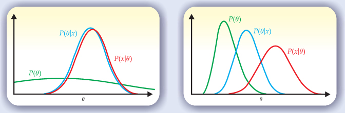
The main idea of Bayesian statistics is to use subjective probability to quantify degree of belief in different models. Bayes’s theorem can be written as P(θ|x) ∝ P(x|θ)P(θ), where, instead of A and B, one has a parameter θ to represent the hypothesis and a data value x to represent the outcome of an observation.

The quantity P(x|θ) on the right-hand side is the probability to obtain x for a given θ. But given empirical data, one can plug the values into P(x|θ) and consider it to be a function of θ. In that case, the function is called the likelihood— the same quantity as mentioned in connection with frequentist methods. The likelihood multiplies P(θ), called the prior probability, which reflects the degree of belief before an experimenter makes measurements. The requirement that P(θ|x) be normalized to unity when integrated over all values of θ determines the constant of proportionality 1/P(x).

The left-hand side of the theorem gives the posterior probability for θ, that is, the probability for θ deduced after seeing the outcome of the measurement x. Bayes’s theorem tells experimenters how to learn from their measurements; the figure presents a couple of graphical examples. But the learning requires an input: a prior degree of belief about the hypothesis, P(θ). Bayesian analysis provides no golden rule for prior probabilities; they might be based on previous measurements, symmetry arguments, or physical intuition. But once they are given, Bayes’s theorem specifies uniquely how those probabilities should change in light of the data.

In many cases of practical interest—for example, a large data sample and only vague initial judgments—Bayesian and frequentist methods yield essentially the same numerical results. Still, the interpretations of those results have subtle but significant differences. In important cases involving small data samples, the differences are apparent both philosophically and numerically.

What you knew and when you knew it

The difficulties in a Bayesian analysis usually stem from the requirement of the prior probabilities. Before measuring a parameter θ, say, a particle mass, one might be tempted to profess ignorance and assign a noninformative prior probability, such as a uniform probability density from 0 to some large mass.

An important problem is that specification of ignorance for a continuous parameter is not unique. For example, a model may be parameterized not by θ but instead by λ = ln θ. A constant probability for one parameter would imply a nonconstant probability for the other. Nevertheless, one often uses uniform prior probabilities not because they represent real prior judgments but because they provide a convenient point of reference.

Difficulties with noninformative priors diminish if one can write down probabilities that rationally reflect prior input. The problem is that judgments of what to incorporate and how to do it can vary widely among individuals, and one would like experimental results to be relevant to the entire scientific community, not just to scientists whose prior probabilities coincide with those of the experimenter. So to be of broader value, a Bayesian analysis needs to show how the posterior probabilities change under a reasonable variation of assumed priors.

Scientists should not be required to label themselves as frequentists or Bayesians. The two approaches answer different but related questions, and a presentation of an experimental result should naturally involve both. Most of the time, one wants to summarize the results of a measurement without explicit reference to prior probabilities; in those cases the frequentist approach will be most visible. It often boils down to reporting the likelihood function or an appropriate summary of it, such as the parameter value for which it is maximized and the standard deviation of that so-called maximum-likelihood estimator.

But if parts of the problem require assignment of probabilities to nonrepeatable phenomena then Bayesian tools will be used. In general, experiments involve systematic uncertainties due to various parameters whose values are not precisely known, but which are assumed not to fluctuate with repeated measurements. If information is available that constrains those parameters, it can be incorporated into prior probabilities and used in Bayes’s theorem.

For many, it is natural to take the results of an experiment and fold in both the likelihood of obtaining the specific data and prior judgments about models or hypotheses. Anyone who follows that approach is thinking like a Bayesian.

The online version of this Quick Study has further resources and examples.

References

1. T. Bayes, Philos. Trans. 53, 370 (1763), https://doi.org/10.1098/rstl.1763.0053
reprinted in Biometrika 45, 293 (1958).2. R. D. Cousins, Am. J. Phys. 63, 398 (1995). https://doi.org/10.1119/1.17901
3. P. Gregory, Bayesian Logical Data Analysis for the Physical Sciences: A Comparative Approach with Mathematica Support, Cambridge U. Press, New York (2005). https://doi.org/10.1017/CBO9780511791277
4. D. S. Sivia with J. Skilling, Data Analysis: A Bayesian Tutorial, 2nd ed., Oxford U. Press, New York (2006).
More about the authors
Glen Cowan is a senior lecturer in the physics department at Royal Holloway, University of London.
Glen Cowan, 1 Royal Holloway, University of London .