The many dimensions of Earth’s landscapes

Humans are born with built-in remote sensing equipment: With our eyes, ears, and noses, we gather information about far-away objects. When we look at a tree and judge its health based on the number and colors of its leaves, we are performing a sort of spectral analysis. The three types of cone cells in the human eye sense light in three spectral bands; the mantis shrimp, with its 16 types of cones, sees, in principle, much more.

Similarly, a digital camera senses three bands, whereas NASA’s Terra and Aqua satellites each carry an instrument called MODIS (Moderate Resolution Imaging Spectroradiometer) that views Earth in 36 bands. The bands sample a spectral region (405 nm–14.4 μm) that ranges from the visible well into the long-wavelength IR. Data from those instruments help researchers to monitor the oceans and land and categorize Earth’s surface into 17 broad classes—for example, savannahs, croplands, and water—frequently called the MODIS land-cover types.

However, multiband instruments leave gaps in the spectrum. Imaging spectrometers fill in those gaps by spanning the wavelength range of interest with hundreds of contiguous bands. The amount of information that can be extracted from an image taken by such an instrument depends on both the spectral diversity of the light coming from a scene and the spectral sensitivity of the instrument.

Several space-based imaging spectrometers are in the works, including one proposed by the Jet Propulsion Laboratory (JPL) called the Hyperspectral Infrared Imager (HyspIRI). ¹ In 2013 NASA and JPL launched the HyspIRI Preparatory Airborne Campaign to demonstrate the capability of such instruments. For the job, they turned to the Airborne Visible/Infrared Imaging Spectrometer (AVIRIS), which has a similar bandwidth and spectral resolution as the instrument planned for HyspIRI. The aim was to take multiple images of large and diverse areas of California that represent all 17 MODIS land-cover types.

To examine the spectral diversity seen in the HyspIRI-preparatory data, JPL’s David Thompson and his colleagues have carried out a statistical analysis of the 2013–14 data set. ² The results portray a California of high spectral diversity that is distributed in distinct ways for different land-cover types.

How much does a camera see?

The spectral diversity captured by an image can be quantified by a value called the intrinsic dimensionality. In essence, it is the number of independent variables necessary to describe a given data set. Digital photographs taken with an RGB camera, for instance, carry at most three dimensions. The number is not always equal to the number of colors; a scene with many colors could have a dimensionality of 1 if all the colors involve a particular linear combination of red, green, and blue.

The AVIRIS detector measures visible to short-wavelength IR spectra (400 nm–2.5 μm) in 224 contiguous, 10-nm-wide spectral bands. In flight, the instrument sweeps a scanning mirror back and forth perpendicular to the direction of the aircraft’s path. ³ When flown at an altitude of 20 km, it has a spatial resolution of about 20 m.

As is the case with other imaging spectrometers, the raw data from AVIRIS come as a data cube; each spatial x–y pixel has a full spectrum along the z-axis. The data that the JPL group used for their analysis included more than 600 flight lines, which they broke into 20 km segments. Each of the more than 4000 segments contains somewhere in the neighborhood of 700 000 spectra. That adds up to nearly 3 × 10⁹ spectra for the entire campaign.

To estimate the dimensionality of a scene, the group used principal-component analysis, a venerable statistical technique that aims to recast a set of possibly correlated independent variables into a new set of uncorrelated variables. Those uncorrelated variables, or principal components, are linear combinations of the wavelength bands ranked in order of their degree of spatial correlation.

The dimensionality is the number of resulting principal components for which the signal is greater than the noise. Consequently, one has to decide what is signal and what is noise. To automate the decision making, Thompson and his colleagues came up with an algorithm that smooths the segment image for each principal component. The signal is taken to be the smoothed data and the noise to be the difference between the smoothed and unsmoothed data.

With that procedure the team obtained the same dimensionality estimates from multiple images—taken months apart under varying illumination—of Ivanpah Playa, a barren, visually unchanging location on the California–Nevada border. That consistency confirmed that the noise-estimation procedure worked as it should and gave the team confidence that seasonal variability seen in croplands, on mountaintops, and for other more mercurial scenes was being correctly determined.

Colorful California

With one of the largest imaging spectroscopy data sets ever collected to hand, Thompson and his colleagues set out to evaluate how dimensionality was distributed for the different land-cover types and to look at its stability over time. In addition, they wanted to check the seemingly intuitive notion that spectral diversity should increase as one goes from scenes of open water to natural environments on land to urban scenes.

The average dimensionalities in individual 20 km segments ranged from single digits to the high 40s. For the complete data set, Thompson and his colleagues estimate a dimensionality of about 50. Geographer Dar Roberts of the University of California, Santa Barbara, says that the HyspIRI Preparatory Airborne Campaign provides a good preview of future satellite-borne missions that will look at the entire surface of Earth. “As diverse as California is, it probably still only represents a fraction of the global diversity,” he says.

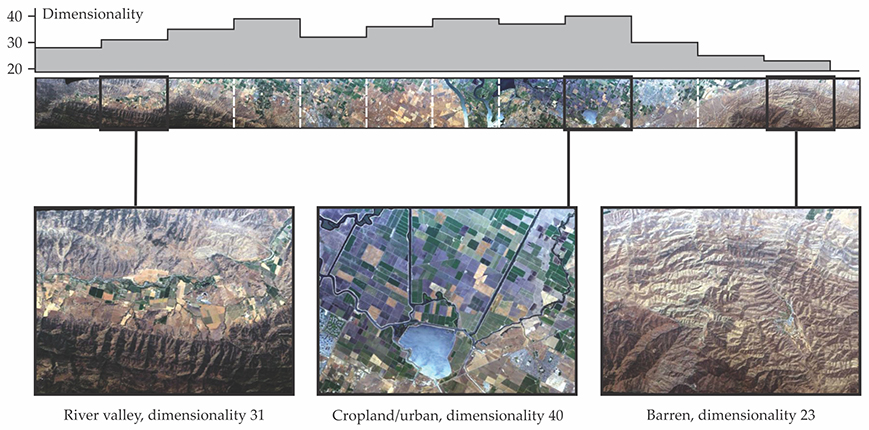
Figure 1 shows a portion of a flight line taken in May 2014 and highlights some representative land-cover types. For some perspective on the dimensionality estimates, consider an RGB digital photograph, which can have at most a dimensionality of 3. In the so-called true-color scheme, those three dimensions, each carrying an integer value between 0 and 255, can encode 256³ or 16 777 216 different colors. The number of distinguishable things grows exponentially with the dimensionality. “Anything raised to the 20th power is already mind-bogglingly high,” Thompson notes. “To the 50th power is even more so.”

A 224-band instrument might therefore seem like overkill for scenes with 50 spectral dimensions. But having more bands than strictly necessary could prove crucial. For a case in point, Thompson uses the normalized difference vegetation index (NDVI). The index is calculated as the ratio of the difference and sum of reflectances measured by two spectral bands—one in the visible and one in the near-IR. It rates the relative greenness of vegetation and is often used as a proxy for plant health. But haze from atmospheric aerosols, surface material near the vegetation, the variety of plants present, and many other factors can affect the ratio. The effects of those factors, explains Thompson, end up as assumptions in models designed to infer meaning from the NDVI. By dint of having so many bands, an imaging spectrometer can measure those confounding details and validate or falsify the models.

Figure 2 shows the dimensionality distribution for three types of scenes. As expected, aquatic scenes, on average, are the least spectrally diverse and urban areas are the most diverse. “When we dig minerals out of the ground and paint them on our cars, that tends to increase the dimensionality,” remarks Thompson. Surprisingly, he says, the segments with the greatest spectral diversity were not in a city but in an agricultural area in southern California’s Imperial Valley. The heavily irrigated region turns out to produce more than a hundred different commodities, including grains, garden vegetables, livestock, and flowers. That variety gives the area a high spectral diversity.

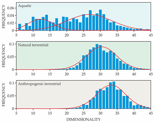
Terrestrial scenes follow a simple Gaussian distribution, with urban areas and croplands having a significantly higher mean dimensionality than forests and other natural settings. Aquatic scenes, however, are better described by a bimodal distribution. Thompson and his colleagues conjecture that the higher dimensional mode may come from segments that contain land features in addition to water.

Colorful future

Imaging spectrometers have been around since the 1980s. The AVIRIS instrument captured its first images in 1987. However, the inherent complexity of the data has presented difficulties. “We’re just now reaching a point where we’ve matured our algorithm savvy and our computer capabilities so that imaging spectroscopy is really becoming accessible in a meaningful way,” says Thompson. He cites the increasing availability of imaging spectroscopy data that have been precorrected for atmospheric effects. With multiple international projects planned to send imaging spectrometers into orbit, says Thompson, “It’s really starting to come into its own and will continue to do so.”

References

1. C. M. Lee et al., Remote Sens. Environ. 167, 6 (2015). https://doi.org/10.1016/j.rse.2015.06.012
2. D. R. Thompson et al., Opt. Express 25, 9186 (2017). https://doi.org/10.1364/OE.25.009186
3. R. O. Green et al., Remote Sens. Environ. 65, 227 (1998). https://doi.org/10.1016/S0034-4257(98)00064-9