Laser Technique Follows Turbulent Flow in Three Dimensions

A simple equation, the Navier–Stokes, completely describes a fluid’s flow. A single parameter, the Reynolds number, flags a flow as smooth or turbulent. But a true understanding of turbulence—one that would furnish accurate predictions of a hurricane’s path or a car’s drag—remains out of reach.

Studying small-scale eddies could bring that goal closer. Tornados and breaking waves look different from afar, but their kinetic energy ends up in the same sort of localized viscous heating. If, as fluid dynamicists suspect, small-scale eddies behave in a universal way before they dissipate, it might be possible to build up reliable predictions of large-scale behavior.

But even if one explored the smallest scales, one property of turbulence blocks the path to understanding: intermittence. In turbulent flows, violent, sporadic jumps can occur without warning. Such events, despite their rarity, can’t be ignored. A once-a-century gust of wind could be the one that blows the roof off your house.

Because of intermittence, hunting for the universal features of turbulence on small scales requires not only high temporal and spatial resolution, but also the ability to gather enough data to capture rare events. And because turbulence is intrinsically anisotropic, one needs to view the flow in three dimensions.

Benjamin Zeff, his thesis adviser Dan Lathrop of the University of Maryland in College Park, and their collaborators have met all these observational challenges in a single experiment. Based around lasers and high-speed video cameras, their apparatus is already shedding light on how two key properties of turbulence, vorticity and dissipation, interact. ¹

Lasers, cameras, action!

The Maryland experiment exploits a generic technique called particle image velocimetry (PIV). In PIV, one seeds a flow with tiny beads that fluoresce or reflect light when illuminated. Various PIV schemes have been developed. Some track single particles as the flow sweeps them along; some use holography to take snapshots of the whole flow. But when Lathrop and Zeff began their project, they found that none of the existing PIV schemes could deliver the long stretches of high-resolution, three-dimensional data they needed.

At first, Lathrop and Zeff thought the answer was straightforward, at least conceptually: Just add fluorescent beads to a tank of water, agitate, illuminate with a laser, then film the flow with high-speed cameras. Looking at motions on the Kolmogorov scale—that is, the scale at which viscosity smoothes the flow—would ensure that the first two terms of a Taylor expansion suffice to describe the flow’s velocity. Working in this linear regime, they reasoned, would simplify the computation and provide all the information they needed about the flow, including the full 3 × 3 velocity gradient matrix.

Zeff originally set to work on a Taylor–Couette tank that Harry Swinney of the University of Texas at Austin had lent to the Maryland team. In a Taylor–Couette tank, fluid that fills the gap between two concentric cylinders is whipped into a turbulent state by the rapid rotation of one or both of the cylinders. Unfortunately, Taylor–Couette flow turned out to be too hard to study on the Kolmogorov scale because the mean flow carried the beads out of the illuminated volume too quickly.

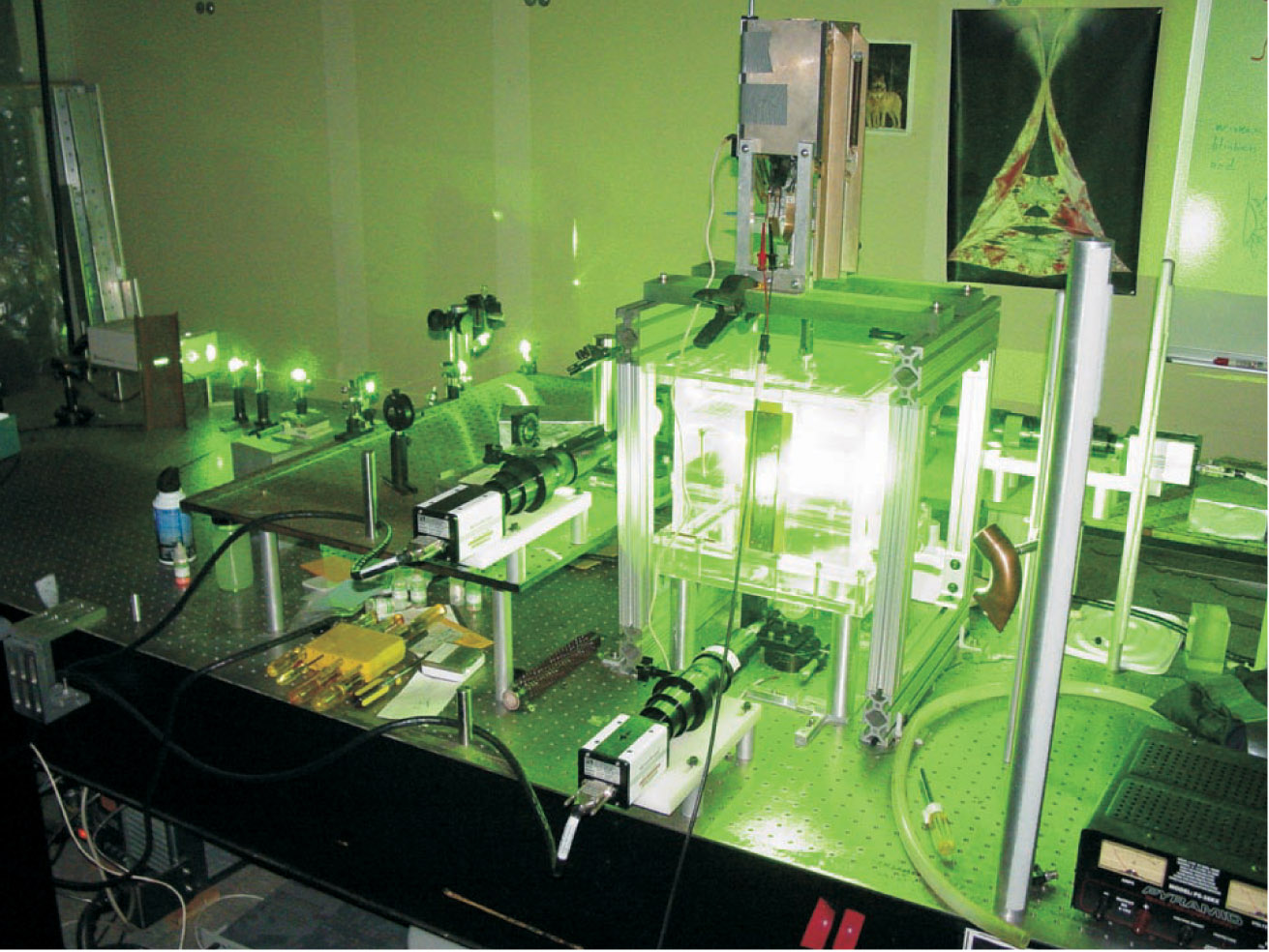
Zeff opted instead to work on another classic exemplar of turbulence, grid turbulence. The setup he developed appears in the above photo. It centers on a cubic tank with transparent acrylic walls, 22 cm on a side, that holds about 10 liters of water and 3 milliliters of 1-micron-sized polystyrene beads. Two horizontal grids, separated by 10 cm, drive the turbulence by oscillating up and down with an amplitude of 0.32 cm and a frequency of 10 Hz. The resulting Reynolds number is a highly turbulent 48 000; the Kolmogorov scale is 0.75 mm.

Illuminating a cubic millimeter of fluid isn’t hard, but Zeff and Lathrop found that their original idea of spotlighting the entire 1 mm³ volume didn’t work. The cameras were unable to tell exactly where the beads were, and so couldn’t yield accurate velocity gradients. Zeff and Lathrop decided instead to illuminate beads passing through and along three of the cube’s intersecting faces.

To create such an illumination pattern, Zeff and Lathrop sought the help of their Maryland colleague and laser expert Raj Roy and his graduate student Ryan McAllister. In the system they built, light from a single continuous-wave laser is split into three mutually orthogonal beams that converge in the center of the tank. One beam points vertically through the bottom of the tank; the other two point horizontally.

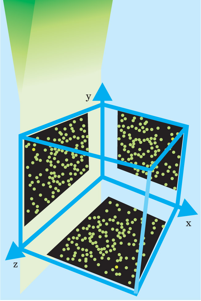
To form the faces of the cube, the beams pass through cylindrical lenses that focus the beam into sheets about 2 mm long and 10 µm thick (see the figure above). Aligning the sheets to intersect proved to be the experiment’s hardest task. Zeff did it by looking at the sheets with the same cameras that imaged the flow. He then repositioned the beams with micrometers.

The Maryland researchers used three cameras, one for each sheet, operating at 125 frames per second. Each camera viewed the flow through microscopes that brought into sharp focus only the sheet in the center of its field of view. After starting the flow, Zeff would run the cameras for 16 seconds (the time it took to fill the cameras’ memory), wait for 48 seconds for the data to be transferred and reduced, then run the cameras again. By adding together data from 2500 such runs, he generated a dataset that occupied almost three terabytes of disk space.

To dig out the physics from such a huge pile of data, the Maryland team turned to an applied mathematician, Eric Kostelich of Arizona State University in Tempe. Kostelich devised an algorithm that compared the beads’ two-dimensional positions from frame to frame to derive, for the flow within the cube, all three components of the velocity and all nine components of the velocity gradient matrix.

The matrix captures much of the physics of the flow. Its symmetric part is proportional to the rate at which the fluid suffers strain, and hence, to the rate of energy dissipation. The antisymmetric part yields a quantity called enstrophy, which is a measure of the flow’s vorticity.

Vortex squelch

Thanks to their trove of data, Lathrop and his colleagues could track how dissipation and vorticity behaved all the way up to 30–40 standard deviations above their respective norms. That the two quantities tended to rise and fall together suggested a picture of how turbulent events unfold. First, stretching occurs and starts to amplify itself and, with it, any vortices that spin about the stretching direction. But when the vortices get too big, they suppress the strain in a process Lathrop calls vortex squelch. The vortices last longer than the stretching, but eventually dissipate.

Lathrop’s mechanism could be an important piece in the turbulence puzzle, but it hardly completes the picture. Lewis Richardson in the 1920s and Andrey Kolmogorov in the 1940s proposed that the path to understanding turbulence lay in following the energy’s course from the large input scale of, say, a ship’s propeller down to the small scale at which viscosity turns energy into heat. Being able to watch that process from beginning to end, with high time resolution and in 3D, is the Golden Fleece of experimental turbulence studies.

Whether the College Park setup can be extended to look at a wider range of length scales is not clear, but it’s already being used to study other problems. Another of Lathrop’s students, Dan Lanterman, is trying to find out why adding polymer molecules to water reduces strain and drag. Fire departments are interested in the answer. They add polymers to reduce the power needed to force water from their hoses.

References

1. B. W. Zeff et al., Nature 421, 146 (2003) https://doi.org/10.1038/nature01334 .
2. B. W. Zeff, “Three-Dimensional Dissipation Scale Measurements of Turbulent Flows,” PhD thesis, U. of Maryland, College Park, 2002. Available at http://complex.umd.edu/INDEX/zeff-phd.pdf .