Ultimate turbulent thermal convection

Thermally driven turbulent flow can be found throughout nature and technology. Such flow transports not only heat but also mass and momentum. Comprehending what determines that transport is key to understanding numerous geophysical and astrophysical flows and to being able to control the industrial and more general flows that people experience every day.

Geophysical flows include the transport of heat in the atmosphere and the ocean, which determines weather, climate, ocean circulation, and the melting of ice shelves. Astrophysical examples include the transport of heat in the core and in the outer layer of stars and planets. Industrial examples include the transport of heat in chemical reactors and in electrolysis and other contexts of energy conversion. At the human scale, people most directly experience heat transport in the buildings, rooms, and vehicles whose temperature they control.

In all those systems, the fundamental question is, How much heat, mass, or momentum is transferred by the system? Direct measurements are difficult to make, as the geometries are often complicated, heat may leak out of the system, the boundary conditions may not be well known or well controlled, and global measurements may not be possible, given the length scales of the systems. What’s more, direct numerical simulations may be prohibitive if the exact experimental boundary conditions are unknown.

Given those difficulties, the aim should be to understand real systems by using simple model systems, from which one can extrapolate the transport properties to the relevant flows. But developing those models requires a deep understanding of the system. That is especially true when the system undergoes a transition from one state to another—from a laminar-like state to a turbulent one, for instance—as then the transport properties of the flow can dramatically change. It is thus key to identify possible transitions between different states in such systems.

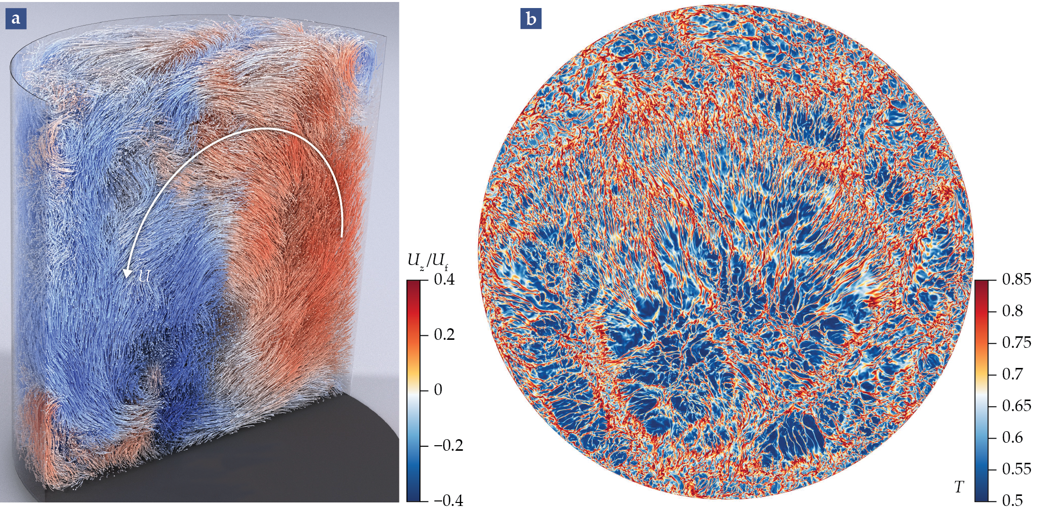
The most famous and most frequently used model to study thermally driven flows is the Rayleigh–Bénard (RB) system. It consists of a flow in a closed box of height $L$, homogeneously heated from below through a hot bottom plate and cooled from above through a cold top plate. The flow is driven by the density differences between the lighter (usually hot) fluid, whose buoyancy makes it rise, and the heavier (usually cold) fluid, which sinks. Figure 1, which shows experimental and numerical snapshots of the flow field for strong thermal driving—to be quantified below—illustrates the complexity of the flow and the large-scale structure that evolves, which is known as the “wind of turbulence” (see the article by Leo Kadanoff, Physics Today, August 2001, page 34 ).

Figure 1.

RB convection has always been a popular playground in which to develop new concepts, such as instabilities, nonlinear dynamics, and the emergence of spatiotemporal chaos and patterns. ¹ For very weak driving, the system has few degrees of freedom—it can be described using few coupled ordinary differential equations—but with increasing driving force it gains more degrees of freedom and eventually becomes turbulent. ^{2 , 3} The RB paradigm applies to heat transfer as well as mass transfer if it is driven by density differences—for example, in a system with heavier salty water at the top and lighter fresh water at the bottom, as can be found in the ocean and in industrial applications.

Several reasons account for the paradigm’s popularity. The underlying dynamical equations—the Navier–Stokes equation, the advection–diffusion equation, and the continuity equation—result from momentum, energy, and mass conservation, respectively. And the respective boundary conditions are well known, so the system is mathematically well defined. The RB system is closed, so that exact global balances between the forcing and the dissipation can be derived. It also has various symmetries, such as temporal and spatial translation symmetries, rotational symmetry, and, for small-enough temperature differences, top–bottom reflection symmetry; they make it attractive for theoretical approaches. And thanks to its simple geometry, the system is accessible to controlled experiments and to direct numerical simulations, provided the thermal driving is not too strong.

Dimensionless numbers

The most relevant question in turbulent RB convection is, How does the heat transport—that is, the time- and area-averaged vertical heat flux (in dimensionless form, the Nusselt number $\mathit{Nu}$, the ratio of convective to conductive heat transfer)—depend on the three dimensionless control parameters of the system? Those parameters are the Rayleigh number $\mathit{Ra}$ (the nondimensionalized temperature difference $\mathrm{\Delta }$ between the hot and cold plates—that is, the thermal driving strength), the Prandtl number $\mathit{Pr}$ (the ratio of the momentum diffusivity to thermal diffusivity), and the aspect ratio $\mathrm{\Gamma }$ (the ratio of the container’s width to its height).

The box above lists some typical values for $\mathit{Ra}$ and $\mathit{Pr}$ in nature and technology. Both $\mathit{Nu}$ and the Reynolds number $\mathit{Re}$ (the ratio of inertial forces to viscous forces) are dependent on $\mathit{Ra}$, $\mathit{Pr}$, and $\mathrm{\Gamma }$. Those dependencies are traditionally sought in the form of scaling laws: $\mathit{Nu}~{\mathit{Ra}}^{\gamma }{\mathit{Pr}}^{\delta }$ and $\mathit{Re}~{\mathit{Ra}}^{\xi }{\mathit{Pr}}^{\eta }$. Researchers have tried to measure and understand those dependencies for at least the last 60 years. ^{2 , 3} And for the past 30 years, they have been helped by direct numerical simulations of the system.

Classical regime

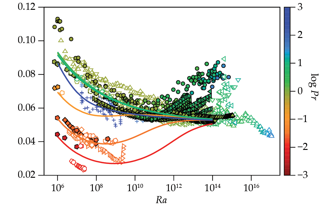
In the regime of Rayleigh numbers up to $\mathit{Ra}$ ~ 10¹¹—which has become feasible in many labs over the past three decades and is nowadays known as the classical regime of turbulent RB convection—researchers have reached broad agreement among various experiments and numerical simulations. Figure 2 shows $\mathit{Nu}(\mathit{Ra},\mathit{Pr})$ for Prandtl numbers varying over six decades, 10⁻³ ≤ $\mathit{Pr}$ ≤ 10³, in cylindrical cells with 1/2 ≲ $\mathrm{\Gamma }$ ≲ 1. Researchers have a good understanding of the regime, thanks to a unifying theoretical approach to wall-bounded turbulence developed by Siegfried Grossmann and one of us (Lohse). ⁴ Called the GL theory, it builds on the ideas of Ludwig Prandtl, Heinrich Blasius, Andrey Kolmogorov, and Sergei Obukhov.

Figure 2.

The unifying theory uses two exact equations, which are straightforwardly obtained by volume integration and the divergence theorem from the Navier–Stokes equations for the velocity field $\mathbf{u}(\mathbf{x},t)$, driven by the buoyancy force from the temperature, and from the advection equation for the temperature field $\theta (\mathbf{x},t)$; here $\mathbf{x}$ denotes spatial coordinates and $t$, time. Assuming that the material properties apart from density are temperature independent, the two equations for the time- and volume-averaged viscous and thermal dissipation rates are, respectively, $${\epsilon }_u\equiv \nu {⟨{({\mathrm{\partial }}_i{u}_j(\mathbf{x},t))}^2⟩}_V=\frac{{\nu }^3}{L^4}(\mathit{Nu}-1)\mathit{Ra}{\mathit{Pr}}^{-2}\text{, and}$$ $${\epsilon }_{\theta }\equiv \kappa {⟨{({\mathrm{\partial }}_i\theta (\mathbf{x},t))}^2⟩}_V=\kappa \frac{{\mathrm{\Delta }}^2}{L^2}\mathit{Nu}\text{.}$$

Those equations are remarkable insofar as they connect volume-averaged quantities (${\epsilon }_u$ and ${\epsilon }_{\theta }$) with the vertical heat transport, $\mathit{Nu}$. The basic assumption of the GL theory is that the physics inside the turbulent core—the bulk of the flow—is fundamentally different from that in the boundary layers (BLs), as shown in figures 3a–3b. Accordingly, the time- and volume-averaged viscous and thermal dissipation rates are composed of two parts, namely (1) $${\epsilon }_u={\epsilon }_{u,\mathrm{BL}}+{\epsilon }_{u,\mathrm{bulk}}$$ $$\text{and}$$ (2) $${\epsilon }_{\theta }={\epsilon }_{\theta ,\mathrm{BL}}+{\epsilon }_{\theta ,\mathrm{bulk}}\text{.}$$

Figure 3.

Because of the differing physics in the bulk and in the boundary layers, their scaling behaviors differ as well. That, in turn, rules out the traditionally assumed pure scaling behavior $\mathit{Nu}~{\mathit{Ra}}^{\gamma }{\mathit{Pr}}^{\delta }$ and $\mathit{Re}~{\mathit{Ra}}^{\xi }{\mathit{Pr}}^{\eta }$ over the full range of $\mathit{Ra}$ and $\mathit{Pr}$.

How do the four individual contributions in equations 1 and 2 scale? In the turbulent bulk, the viscous and thermal dissipation rates ${\epsilon }_{u,\mathrm{bulk}}$ and ${\epsilon }_{\theta ,\mathrm{bulk}}$ follow the 1941 Kolmogorov–Obukhov scaling relations for turbulent flow (Kolmogorov turbulence). In terms of the turbulent wind velocity $U$ and the temperature difference $\mathrm{\Delta }$ between the plates, those relations imply that ${\epsilon }_{u,\mathrm{bulk}}~U^3/L$ and ${\epsilon }_{\theta ,\mathrm{bulk}}~{\mathrm{\Delta }}^{2}U/L$. Those scaling relations cannot hold in the boundary layers near the walls, where viscosity and thermal diffusivity matter. There, as long as the driving is not too strong, the viscous and thermal dissipation rates ${\epsilon }_{u,\mathrm{BL}}$ and ${\epsilon }_{\theta ,\mathrm{BL}}$ scale according to the Prandtl–Blasius theory for laminar-type boundary layers that develop along a solid horizontal plate when a fluid flow has relatively low velocity. (See the article by John D. Anderson Jr, Physics Today, December 2005, page 42 .)

The splitting of wall-bounded turbulent flow into two regions in equations 1 and 2 can be understood by analogy to Prandtl’s foundational insight from 1904 that the potential, or Bernoulli, flow around a plate cannot hold close to the plate itself but must be matched to boundary layers with quite different physics and scaling relations. Only with that insight could Prandtl have obtained the observed Reynolds-number dependence of the drag, as shown in figures 3d–3f. The GL theory follows the same spirit, but for wall-bounded turbulent flow, the outer flow is not of the Bernoulli type but of the Kolmogorov–Obukhov type.

The details of the GL theory are worked out in references and . The theory describes the experimentally and numerically observed dependencies $\mathit{Nu}(\mathit{Ra},\mathit{Pr})$ and $\mathit{Re}(\mathit{Ra},\mathit{Pr})$ over six orders of magnitude in $\mathit{Ra}$ and in $\mathit{Pr}$ up to $\mathit{Ra}$ of about 10¹¹. The theory has proven its predictive power for $\mathit{Ra}$ and $\mathit{Pr}$ parameter ranges for which measurements were carried out only later. The team of Ke-Qing Xia (Chinese University of Hong Kong) measured for large $\mathit{Pr}$ values, and the teams of Sven Eckert (Helmholtz Center Dresden-Rossendorf), Peter Frick (Polytechnical University of Perm), and Jonathan Aurnou (UCLA) measured for small ones.

The key idea of the GL theory—namely, to start from exact global balance equations and to split the dissipation rates into boundary-layer and bulk contributions—is quite general. It has also been applied successfully to various other turbulent flows, such as internally heated turbulence, double-diffusive convection—in which the flow velocity is coupled to both the temperature and the salinity—horizontal convection, and magnetohydrodynamically driven turbulence.

Experiments at large $\mathit{Ra}$

For very large thermal driving beyond $\mathit{Ra}$ ~ 10¹¹, the experimental results for $\mathit{Nu}(\mathit{Ra},\mathit{Pr})$ seem to contradict each other, as shown in figure 2: For very similar $\mathit{Pr}$, the $\mathit{Nu}(\mathit{Ra})$ dependencies are quite different in different experiments. For those large $\mathit{Ra}$, direct numerical simulations become increasingly difficult to perform because of the many degrees of freedom in the system; extremely fine computational grids are required to run the simulations. For many applications, including those in geological and astrophysical contexts, however, the large-$\mathit{Ra}$ limit is of particular interest. So how can one extrapolate insights from the lab scale and numerical simulations at smaller $\mathit{Ra}$ and estimate the heat transport and the turbulence intensity on geo- and astrophysical scales? And how can one perform experiments for very large values of $\mathit{Ra}$ in order to scale up the RB system?

To open the large-$\mathit{Ra}$ regime to experimental studies, the University of Chicago’s Albert Libchaber and colleagues used helium gas close to its critical point in an RB system, as it has extremely low kinematic viscosity and thermal conductivity. In 1989 he and his coworkers ⁵ achieved $\mathit{Ra}$ ~ 10¹⁴. Bernard Castaing, Philippe Roche, and coworkers in Grenoble, France, continued to pursue that line of research. In 1997, Castaing and his collaborators ⁶ found a transition around $\mathit{Ra}$ ~ 10¹¹ toward a steeper effective scaling of roughly $\mathit{Nu}~{\mathit{Ra}}^{0.38}$, much larger than has been seen at lower $\mathit{Ra}$, where the effective scaling exponent never exceeds ⅓. They termed that new regime “ultimate.”

In later work, Roche and his colleagues found the transition Rayleigh number to vary up to $\mathit{Ra}$ ~ 10¹³, depending mainly on the aspect ratio of the cell and the Prandtl number. ⁷ The transition was also evidenced by the buildup of fluctuations in the boundary layer at the same transition Rayleigh number, supporting the view that the transition is connected with a destabilization of the boundary layer—meaning that in the new regime, the flow in the bulk and in the boundary layers are both turbulent.

Russell Donnelly and coworkers at the University of Oregon followed Libchaber’s path of using helium gas as the working fluid close to its critical point, ⁸ but they increased the height of the RB cell and achieved an even larger $\mathit{Ra}$, up to ~ 10¹⁵. In those experiments, however, no transition to a regime with enhanced scaling dependence for $\mathit{Nu}$ could be identified. Nor was there evidence for an enhanced scaling regime in team members’ follow-up experiments, carried out by Joseph Niemela and Katepalli Sreenivasan ⁹ and by Ladislav Skrbek and coworkers. ¹⁰

Guenter Ahlers and Eberhard Bodenschatz proposed another idea for how to achieve very large $\mathit{Ra}$—namely, to use pressurized sulfur hexafluoride as the working fluid. The advantage of using pressurized SF₆ in RB experiments is that over a very large $\mathit{Ra}$ range the system keeps roughly the same $\mathit{Pr}$. Ahlers, Bodenschatz, and coworkers at the Max Planck Institute for Dynamics and Self-Organization in Göttingen, Germany, performed their experiments with SF₆ pressurized up to 19 bars, for which $\mathit{Pr}$ remains roughly 0.7. In 2012 they observed a transition to an ultimate RB regime around $\mathit{Ra}$ ~ 10¹⁴ and with an aspect-ratio dependence consistent with the Grenoble results. The $\mathit{Nu}$ dependence on $\mathit{Ra}$ was steeper above the transition than below it and can be described with an effective scaling law $\mathit{Nu}~{\mathit{Ra}}^{0.38}$ (see reference and later papers by the Göttingen group). The sharp transition was found not only for $\mathit{Nu}$ but also for $\mathit{Re}$ and consistently at the same $\mathit{Ra}$. That observation also supports the view of a fundamental flow transition in an RB cell.

The discrepancy in the large-$\mathit{Ra}$ regime between a typical Grenoble data set (with a transition toward an enhanced scaling around $\mathit{Ra}$ ~ 10¹¹), a typical Oregon data set (without a transition), and a typical Göttingen data set (with a transition around $\mathit{Ra}$ ~ 10¹⁴) can be seen in figure 2. What is the origin of those different findings in the large-$\mathit{Ra}$ experiments, even for very similar control parameters? At the moment, that’s an open question.

Ultimate turbulence regime

What do theories suggest about the existence of an ultimate regime? As early as 1962, Robert Kraichnan proposed an ultimate regime of RB convection ¹² and assumed a fully turbulent boundary layer and a certain scaling relation between $\mathit{Nu}$ and $\mathit{Re}$ for that boundary layer. He obtained $\mathit{Nu}~{\mathit{Ra}}^{\mathrm{½}}{\mathit{Pr}}^{\mathrm{½}}$, with logarithmic corrections. Note that in the ultimate regime, in no case can $\mathit{Nu}$ grow faster than $~{\mathit{Ra}}^{\mathrm{½}}$. That upper bound, which is much larger than any experimental or numerical data for $\mathit{Nu}$, was rigorously proved ¹³ by Louis N. Howard in 1963, with $\mathit{Nu}-1\le C{\mathit{Ra}}^{\mathrm{½}}$, in which $C$ is the constant $\sqrt{3}/8$. Other researchers verified the upper bound for slightly smaller values of $C$ later. ¹⁴

The GL theory of thermal convection ⁴ also suggests an ultimate regime: For large-enough driving strength, the laminar Prandtl–Blasius boundary layers, shown in figure 3a, should become unstable and undergo a transition toward turbulent boundary layers, the so-called Prandtl–von Kármán boundary layers (figure 3b). The transition is a direct analogue of the laminar-to-turbulent transitions of the boundary layers around a plate, as shown in figures 3d–3e or within a pipe. Those transitions are subcritical—meaning that around the transition different states coexist—and have a so-called nonnormal and nonlinear character, where nonnormal refers to the eigenvectors of the linear operator being nonorthogonal. Such transitions have a double-threshold behavior: They can arise when the shear is sufficiently strong and disturbances (such as small wall roughnesses or thermal inhomogeneities in the plates) are large enough to trigger the onset. ¹⁵

Typically, such an onset of shear instability in wall-parallel flow happens when the shear Reynolds number ${\mathit{Re}}_{\mathrm{s}}$ exceeds a value of about 420, as estimated by Walter Tollmien almost a century ago. The GL theory adopts Tollmien’s value as a typical guideline for the onset of the shear instability (for $\mathrm{\Gamma }$ ~ 1), although, of course, in the case of RB flow in a box, the flow is not strictly parallel to the wall. For $\mathit{Pr}$ ≈ 0.7 and $\mathrm{\Gamma }$ ~ 1, the critical Rayleigh number for the onset of the ultimate regime in RB convection ⁴ can be estimated to be around 10¹⁴. But given the double-threshold feature of the transition, it may also be earlier or later for different small disturbances. For larger $\mathit{Pr}$ or smaller $\mathrm{\Gamma }$, the critical Rayleigh number increases.

What dependence $\mathit{Nu}(\mathit{Ra},\mathit{Pr})$ should be expected in the ultimate regime? From an integration of the energy-dissipation rate in the turbulent boundary layer, ¹⁶ one obtains $\mathit{Nu}~{\mathit{Ra}}^{\mathrm{½}}{\mathit{Pr}}^{\mathrm{½}}/{(\log (\mathit{Ra}))}^2$, which in today’s experimentally accessible regime implies an effective scaling of roughly $\mathit{Nu}~{\mathit{Ra}}^{0.38}$.

How then can one reconcile the various seemingly contradictory measurements of $\mathit{Nu}(\mathit{Ra},\mathit{Pr})$ for $\mathit{Ra}$ > 10¹¹, evident in figure 2? The analogy to pipe flow or other shear flows has been helpful to researchers, and over the past few years, they have made some intriguing suggestions as to why the Rayleigh numbers of the observed transitions to the ultimate regime depend on details of the different experiments. The key idea, proposed by Roche in 2020, ⁷ is to realize the subcritical nature of the transition, which has the above-mentioned double-threshold behavior and is the typical feature of transitions in shear flows, ¹⁵ applies in this case because of the strong local shear at the boundaries.

The subcritical nature of the transition implies that multiple states can coexist and that the transition is hysteretic—it depends on the system’s history—and that for strong-enough shear, even quite small disturbances can trigger the transition from laminar flow to turbulent flow (notice the analogy between figure 3c and figure 3f). That interpretation has the potential to reconcile the various observations and different values of the Rayleigh number at which the transition occurs.

Although the transition toward an ultimate turbulence regime for RB turbulence is under intense discussion, no one disputes its relevance for Taylor–Couette (TC) turbulence. ¹⁷ The TC system—two coaxial corotating or counterrotating cylinders with fluid between them—is sometimes called the twin of the RB configuration because of many similarities between the two systems. ¹⁸ The analogy between RB and TC also holds in the ultimate regime and has been observed in all of the experiments and numerical simulations of turbulent TC flow made at large-enough driving strength.

That large-enough driving strength is more easily accessible in TC flow than in RB flow reflects the fact that the mechanical driving in TC flow is much more effective than the thermal driving in RB flow. Similarly, one should also expect an ultimate regime in pipe flow, horizontal convection, and other systems. Were the existence of an ultimate regime doubted in any of those flows, then one would have to come up with a mechanism by which the laminar flow in the boundary layers would remain laminar at arbitrarily large driving strength and the transition to turbulence would be suppressed. Frankly, we do not see what such a mechanism could be.

How then can the controversy on the ultimate regime in RB flow be settled? Given that striving toward ever-larger experiments and numerical simulations is extremely difficult and costly, one possibly promising route is to further explore the analogy to the laminar-to-turbulent transition in flow around a plate, illustrated in figure 3, or in pipe flow. In both cases a detailed analysis of the lifetime of disturbances of different strength has led researchers to conclude that the transition can be interpreted as a directed percolation transition. ¹⁵ Such a transition is quite universal in physics, and it also applies, for example, to epidemiological models for the spreading of diseases. One can hope that analogous experiments, as in pipe flow, and corresponding numerical simulations—including those in which Prandtl numbers vary—will further elucidate the fascinating transition to the ultimate regime.

The issue is of utmost relevance: Researchers must understand how to extrapolate the heat flux from controlled lab-scale experiments to the scales relevant in geophysical contexts. Whether a transition to an ultimate regime occurs or not will change the heat flux by orders of magnitude. But climate models and models for heat circulation in the ocean—with their implications for melting glaciers, nutrition transport, and the prediction of tipping points—clearly require more precision and reliability.

The scientific insights conveyed in this article come from more than three decades of collaborations and interactions with colleagues, postdocs, and doctoral students. We thank all of them for their contributions and for the intellectual pleasure we have enjoyed while working together. We thank Dennis van Gils for help with the figures.

References

1. 1. E. Bodenschatz, W. Pesch, G. Ahlers, Annu. Rev. Fluid Mech. 32, 709 (2000). https://doi.org/10.1146/annurev.fluid.32.1.709
2. 2. G. Ahlers, S. Grossmann, D. Lohse, Rev. Mod. Phys. 81, 503 (2009). https://doi.org/10.1103/RevModPhys.81.503
3. 3. D. Lohse, K.-Q. Xia, Annu. Rev. Fluid Mech. 42, 335 (2010); https://doi.org/10.1146/annurev.fluid.010908.165152
F. Chillà, J. Schumacher, Eur. Phys. J. E 35, 58 (2012); https://doi.org/10.1140/epje/i2012-12058-1
K.-Q. Xia, Theor. Appl. Mech. Lett. 3, 052001 (2013); https://doi.org/10.1063/2.1305201
O. Shishkina, Phys. Rev. Fluids 6, 090502 (2021). https://doi.org/10.1103/PhysRevFluids.6.090502
4. 4. S. Grossmann, D. Lohse, J. Fluid Mech. 407, 27 (2000); https://doi.org/10.1017/S0022112099007545
S. Grossmann, D. Lohse, Phys. Rev. Lett. 86, 3316 (2001); https://doi.org/10.1103/PhysRevLett.86.3316
R. J. A. M. Stevens et al., J. Fluid Mech. 730, 295 (2013). https://doi.org/10.1017/jfm.2013.298
5. 5. B. Castaing et al., J. Fluid Mech. 204, 1 (1989). https://doi.org/10.1017/S0022112089001643
6. 6. X. Chavanne et al., Phys. Rev. Lett. 79, 3648 (1997). https://doi.org/10.1103/PhysRevLett.79.3648
7. 7. P.-E. Roche, New J. Phys. 22, 073056 (2020); https://doi.org/10.1088/1367-2630/ab9449
P.-E. Roche et al., New J. Phys. 12, 085014 (2010). https://doi.org/10.1088/1367-2630/12/8/085014
8. 8. J. J. Niemela et al., Nature 404, 837 (2000). https://doi.org/10.1038/35009036
9. 9. J. J. Niemela, K. R. Sreenivasan, J. Fluid Mech. 481, 355 (2003). https://doi.org/10.1017/S0022112003004087
10. 10. P. Urban et al., New J. Phys. 16, 053042 (2014). https://doi.org/10.1088/1367-2630/16/5/053042
11. 11. G. Ahlers et al., New J. Phys. 14, 103012 (2012); https://doi.org/10.1088/1367-2630/14/10/103012
X. He et al., Phys. Rev. Lett. 108, 024502 (2012). https://doi.org/10.1103/PhysRevLett.108.024502
12. 12. R. H. Kraichnan, Phys. Fluids 5, 1374 (1962). https://doi.org/10.1063/1.1706533
13. 13. L. N. Howard, J. Fluid Mech. 17, 405 (1963). https://doi.org/10.1017/S0022112063001427
14. 14. F. H. Busse, Rep. Prog. Phys. 41, 1929 (1978); https://doi.org/10.1088/0034-4885/41/12/003
C. R. Doering, P. Constantin, Phys. Rev. E 53, 5957 (1996). https://doi.org/10.1103/PhysRevE.53.5957
15. 15. P. Manneville, Mech. Eng. Rev. 3, 15-00684 (2016); https://doi.org/10.1299/mer.15-00684
M. Avila, D. Barkley, B. Hof, Annu. Rev. Fluid Mech. 55, 575 (2023). https://doi.org/10.1146/annurev-fluid-120720-025957
16. 16. S. Grossmann, D. Lohse, Phys. Fluids 23, 045108 (2011). https://doi.org/10.1063/1.3582362
17. 17. S. Grossmann, D. Lohse, C. Sun, Annu. Rev. Fluid Mech. 48, 53 (2016). https://doi.org/10.1146/annurev-fluid-122414-034353
18. 18. F. H. Busse, Physics 5, 4 (2012). https://doi.org/10.1103/Physics.5.4
More about the Authors
Detlef Lohse (d.lohse@utwente.nl) is the chair of the physics of fluids group at the University of Twente in Enschede, the Netherlands. Olga Shishkina (olga.shishkina@ds.mpg.de) is group leader at the Max Planck Institute for Dynamics and Self-Organization in Göttingen, Germany.
This Content Appeared In
pt_cover1123.jpg
Volume 76, Number 11
Related content
/
Article
Technical knowledge and skills are only some of the considerations that managers have when hiring physical scientists. Soft skills, in particular communication, are also high on the list.
Professional societies can foster a sense of belonging and offer early-career scientists opportunities to give back to their community.
Research exchanges between US and Soviet scientists during the second half of the 20th century may be instructive for navigating today’s debates on scientific collaboration.
The Eisenhower administration dismissed the director of the National Bureau of Standards in 1953. Suspecting political interference with the agency’s research, scientists fought back—and won.
Alternative undergraduate physics courses expand access to students and address socioeconomic barriers that prevent many of them from entering physics and engineering fields. The courses also help all students develop quantitative skills.
Defying the often-perceived incompatibility between the two subjects, some physicists are using poetry to communicate science and to explore the human side of their work.
Get PT in your inbox
Physics Today - The Week in Physics
The Week in Physics" is likely a reference to the regular updates or summaries of new physics research, such as those found in publications like Physics Today from AIP Publishing or on news aggregators like Phys.org.
Physics Today - Table of Contents
Physics Today - Whitepapers & Webinars
By signing up you agree to allow AIP to send you email newsletters. You further agree to our privacy policy and terms of service.