The topology of data

A wealth of complex data is increasingly available in almost every aspect of the physical and social world. Such copious data offer the potential to help unlock new ways of understanding and manipulating our surroundings. The demographic characteristics of human populations convey information about heterogeneous regions of a city or a country, and our online activities encode data about who we are and what we do. Networked systems—in people, cities, animals, plants, computers, and more—are also rich in data, which are present both in their structure and in their dynamics. The flows of nutrients in vascular structures, the complicated dynamics of fluids, and the forces in granular materials all provide huge amounts of complex data. Parsing—and hopefully eventually understanding—such data requires a diverse set of tools.

One family of tools, called topological data analysis (TDA), employs ideas from the mathematical field of algebraic topology. Algebraic topology gives a framework to rigorously and quantitatively describe the global structure of a space. By building on and adapting this framework, researchers in physics and many other disciplines are increasingly using TDA to examine how the “shape” of data changes when one views a system at different scales. ² TDA has led to fascinating insights in biophysics, granular materials, fluid dynamics, and many other areas. It has been used to study phase transitions, ³ temperature fluctuations in the cosmic microwave background, ⁴ chaotic behavior in nonlinear dynamical systems, ⁵ and much more. ⁶

In this article, we present a few examples of TDA in condensed-matter and soft-matter physics. We hope that this small selection of TDA research in physics will help illustrate the flavor of insights that one can obtain by applying a topological lens to data.

A few ideas from topology

Topology is a branch of mathematics that concerns the shapes of objects. ¹ It provides a framework that describes the properties of an object that stay the same if we stretch it, shrink it, or bend it without any tearing or gluing. Consider a circular rubber band. Because we can stretch the rubber band into an oval, the circle and the oval are topologically equivalent. However, the rubber band is not topologically equivalent to a segment of a string: The circular rubber band has a hole in the middle, but the string does not.

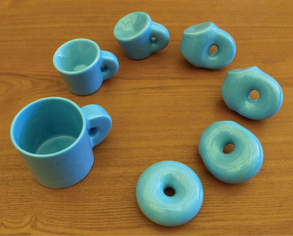
An important aspect of topology is the characterization of the connectedness of objects by counting their numbers of pieces and numbers of holes. Researchers use that information to group objects into different types. For example, a doughnut has the same number of holes and the same number of pieces as a coffee cup with one handle (see figure 1), but it is different from a filled sphere, which has the same number of pieces but does not have any holes.

Figure 1.

Algebraic topology gives a framework to rigorously and quantitatively describe the global structure of a space. Methods for characterizing the global structure of a topological space and objects within it rely on information about the entire space. If we look at a neighborhood of any point on a sphere, we obtain a surface with the same properties as a plane. By zooming in extremely closely, we no longer notice the sphere’s curvature. To a human standing on a very large sphere, such as a planet, the surface appears to be flat. We recover the fact that the sphere has curvature by considering all of its neighborhoods, but we still don’t pick up whether there’s a void inside the sphere. To fully characterize the structure of a sphere, we need to consider the entire sphere at once.

To consider an entire object at once, we use the algebraic-topology concept of homology, which allows us to distinguish between objects based on their numbers and types of “holes.” To make this distinction, we need the notion of a topological space X. Such a space consists of a set of points, along with neighborhoods of each point, that satisfy certain axioms that relate them. ¹ Intuitively, we consider neighborhoods of a certain size around each point and define what it means for the points to be “close” to each other based on whether their neighborhoods overlap. We do not require a numerical value to quantify that closeness; we just need to know when neighborhoods overlap. This gives crucial flexibility for using topological tools in applications. ²

To develop an understanding of homology, it helps to be more precise. The homology of a topological space X is a set of topological invariants that are represented by homology groups H_k(X), which describe k-dimensional holes in X. The rank of H_k(X) is called the Betti number; it is analogous to the dimension of a vector space and counts the number of k-dimensional holes. A feature in H₀ is zero-dimensional and can be visualized as a point; the rank of H₀ is the number of distinct connected components in X. Similarly, a feature in H₁ is one-dimensional and can be visualized as a cycle (that is, a loop). A feature in H₂ is two-dimensional and can be visualized as a cavity. Researchers also examine H_k for larger values of k, but it is harder to visualize the associated features.

Returning to our filled sphere and our coffee cup, the sphere consists of one connected component and zero 1D holes—that is, no cycles—so rank(H₀) = 1 and rank(H₁) = 0; its zeroth Betti number is 1 and its first Betti number is 0. By contrast, a coffee cup has rank(H₀) = 1 and, because of its 1D hole, it has rank(H₁) = 1. We can also use homology to distinguish between a filled sphere and a spherical shell. The former does not have a cavity, so rank(H₂) = 0, but the latter does, so rank(H₂) = 1.

The shape of data

To identify “holes” in a data set and thereby describe its topological “shape,” we need to assign a topological structure to the data and compute topological invariants. Homology groups are good invariants because there are efficient algorithms to compute them.

The most widely used tool in TDA is persistent homology (PH). In PH, one examines homologies across the scales of a data set. ^{2 , 7} Traditionally, one interprets topological features, such as cycles or cavities, that exist for a large range of scales—that is, persistent features—as genuine features of a data set and topological features that exist for only a small range of scales as noise.

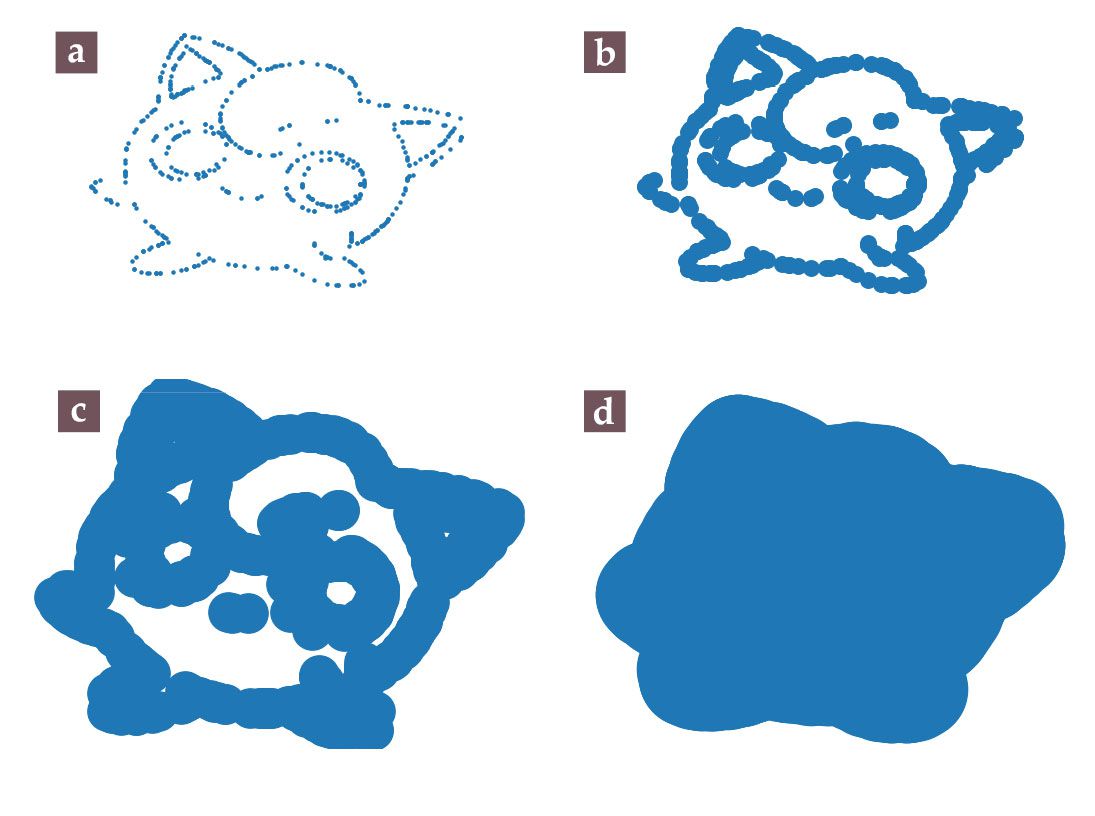
To introduce the main idea of PH, let’s start with a collection of dots (see figure 2). Such an object, called a point cloud, is commonly studied in TDA. ² Point clouds have an inherent 0D structure, and they thus have few interesting topological properties when viewed as a finite collection of points. We now place a ball of some radius ε around each point. The scaling parameter ε, which is sometimes called a filtration parameter, allows us to encode geometric information. The balls fill in areas between points that are close to each other. Essentially, we are squinting at a point cloud so that it blurs and takes some shape. The harder we squint—that is, as we increase the value of ε—the more the boundaries of the shape blur and expand. Points that start out as distinct begin to overlap with each other as ε increases, so the notion of what it means to be “close” changes.

Figure 2.

Figure 2 demonstrates this idea with the Pokémon known as Jigglypuff. Jigglypuff starts out as a collection of dots—that is, a point cloud (figure 2a). As we increase the radius ε of the dots, progressively more of them overlap (figure 2b), and it becomes easier to identify Jigglypuff. As we continue increasing the radius of the dots, Jigglypuff has progressively fewer components (that is, rank(H₀) decreases) and develops some 1D holes (that is, rank(H₁) increases). As ε becomes larger, some holes also disappear (figure 2c), and it becomes harder to identify Jigglypuff. Eventually, when ε becomes sufficiently large, all of the holes disappear (figure 2d). We can see different features of Jigglypuff at different values of ε. A topological feature is “born” at the value of ε at which it first appears and “dies” at the value of ε at which it disappears.

The images in figure 2 demonstrate how the topological features that one obtains from a point cloud change as one views them at different scales. To examine the features systematically, one constructs a computationally convenient mathematical object from such images. ⁷ One such object is a filtered simplicial complex, which is a sequence of simplicial complexes that are nested inside each other. A simplicial complex is a space that is built from a union of points, edges, triangles, tetrahedra, and higher-dimensional polytopes. (A polytope is a geometric object with flat faces and edges; it is a generalization of polygons and polyhedra to any number of dimensions.) The word “filtered” describes how simplicial complexes nest inside each other as one varies some parameter, such as the radius of the dots in figure 2.

Simplicial complexes are topological spaces that one can use to approximate other topological spaces in a way that captures their topological properties. For example, a tetrahedron can approximate a sphere. There are many choices for how to construct a filtered simplicial complex. For instance, in figure 2, the simplicial complex is based on distance (the dot size). For a given application, it is desirable to choose a construction that satisfies the intuition that genuine features are also persistent features.

The extension of homology to PH allows us to quantify holes in data in a meaningful way. We are interested in persistent holes (and other persistent features), such as Jigglypuff’s eyes in figure 2, that exist for a large range of values of an adjustable parameter. When studying physical systems, it is desirable for the parameter to correspond to something physical. Such homological ideas have been used to analyze data sets in many applications. ^{2 , 7} The computation of PH has been especially prominent in neuroscience, ⁸ and it has also been used in areas such as granular physics, fluid dynamics, nonlinear dynamics, cosmology, string theory, and computer vision.

Introductions to PH and to TDA more generally are available for a variety of audiences. See reference for an introduction to TDA and PH for teenagers and preteens, reference for a recent review of TDA for a general physics audience, and reference for a classic textbook on the mathematics of TDA. Reference overviews PH and gives an introduction to the installation, use, and benchmarking of several software packages for it.

Amorphous and granular matter

TDA has yielded many insights into granular and amorphous matter. Notions of connectivity and gaps are natural in such systems, ¹⁰ and they relate to important physical ideas, such as which parts of a system will fail first and which physical quantities to measure to forecast the onset of failure. They are also relevant for obtaining insights into packing, jamming, and characterizing the different states of a system.

Lou Kondic and colleagues used PH to track how simulations of 2D granular force networks—sets of interparticle contacts that carry loads that are larger than the mean load of a system—evolve as a system crosses a jamming point. ¹¹ They used the interparticle force as a filtration parameter. To compute H₀, they determined the distinct components of mutually contacting particles that experience forces above that force. They associated the jamming transition with a sudden large increase in the number of components, and hence in rank(H₀), above a threshold force that approximately equals the mean interparticle force in the system. Computing H₀ and H₁ also allows one to quantitatively describe the effects of bidispersity and polydispersity (the presence of particles of three or more sizes) and friction on the structure of granular force networks. In other studies, TDA was used to examine changes in the structure of polydisperse granular materials with packing fraction, the effect of compression on the relative prevalence of branching and compact regions in granular force networks, and more. ¹⁰

In a recent study, Jason Rocks and colleagues used PH to systematically explore “softness” in amorphous packings of particles. ¹² Notions of softness capture the propensity of particles to rearrange structurally. A good measure of softness should allow one to forecast structural rearrangements of particles. Using the approach that we illustrate in figure 3, Rocks and colleagues examined the topological structures of configurations at the onset of particle rearrangements in bidisperse particle packings and obtained interpretable, topologically informed descriptions of packing structure that are experimentally measurable.

Figure 3.

Consider the 2D packing of circular particles in figure 3a. We construct a distance-based simplicial complex that is known as an alpha complex. At the center of each particle i, we place a disk of radius r_i(α) = (R_i² + α)^1/2, where R_i is the radius of particle i and α is the filtration parameter. In essence, α is an interaction radius. When α > 0, the disks are larger than their corresponding particles; when α < 0, the disks are smaller than their associated particles. For the smallest value of α, we obtain figure 3b. At that minimum interaction radius, we have a point cloud.

The simplicial complex that corresponds to figure 3b consists of a set of nodes; these are the particle centers. There are no edges, triangles, or higher-dimensional polytopes that connect interacting particles. As we increase α, some of the disks overlap, and we add the associated polytopes to the alpha complex. Analogously to what we saw for Jigglypuff in figure 2, 1D holes are born (see figure 3c) and then eventually die (see figure 3d) as α increases.

A persistence diagram (PD) summarizes the births and deaths of topological features as a function of a filtration parameter. The PD in figure 3e conveys the births and deaths of 1D holes for progressively larger values of α. The horizontal axis of a PD indicates the filtration parameter values α_b at which features are born, and the vertical axis indicates the values α_d at which they die. Features that live longer—that is, that are more persistent—lie farther above the diagonal line.

Rocks and colleagues used PDs to quantify the topological structure of jammed packings and to connect that structure with dynamics. ¹² Cycles—that is, 1D holes—play an important role in their topologically informed descriptions of packing structure. The birth value α_b measures the length of the longest edge in a cycle, and the death value α_d indicates the scale of the cycle in a packing. The researchers examined PDs for a range of system configurations. The birth and death values of cycles helped them examine the presence and absence of gaps between particles, which in turn allowed them to quantify local rearrangements of particles. The longest edge of a cycle with α_b < 0 corresponds to a contact between particles, so such a cycle consists only of contacts. By contrast, the longest edge of a cycle with α_b > 0 corresponds to a gap between particles; such a cycle may also include some contacts. The more gaps—and, hence, fewer contacts—that a particle has with its nearest neighbors, the more it participates in local rearrangements.

TDA can also help illuminate phase transitions, such as those between amorphous solids and other states. In amorphous solids—which include glasses, plastics, and gels—the atoms and molecules are not organized as a lattice. In a recent study of particle configurations in amorphous solids, Yasuaki Hiraoka and colleagues computed PH in random networks and random packings that they generated from molecular-dynamics simulations of various systems, including silica glass and copper–zirconium metallic glass. ¹³ They examined hierarchical structures in the systems by using PDs to characterize 1D and 2D homological features. They found that such topological features can clearly distinguish amorphous-solid states from liquid and crystalline states.

Vascular networks

From the unicellular and multinucleate slime mold Physarum polycephalum to the xylems of leaves and the circulatory systems of animals, vascular networks permeate every large-scale organism. The structure of a vascular network affects numerous crucial phenomena, such as the flow of water and other liquids, the distribution of nutrients in organisms, and the pressure distributions that drive nutrient flow. TDA is a valuable approach to study the properties of vascular networks and relate them to network function. For example, the computation of PH offers a potential tool for the early detection of subtle changes in microvasculature that can signify the onset of disease.

Vascular networks have hierarchical features (see figure 4) and are often dominated by cycles, which help determine system organization. Vein-width histograms and other prevalent tools to quantify the structure of vascular networks do not capture the hierarchical nature of their connectivity. Topological approaches, however, are able to uncover intricacies in the networks’ hierarchical organization.

Figure 4.

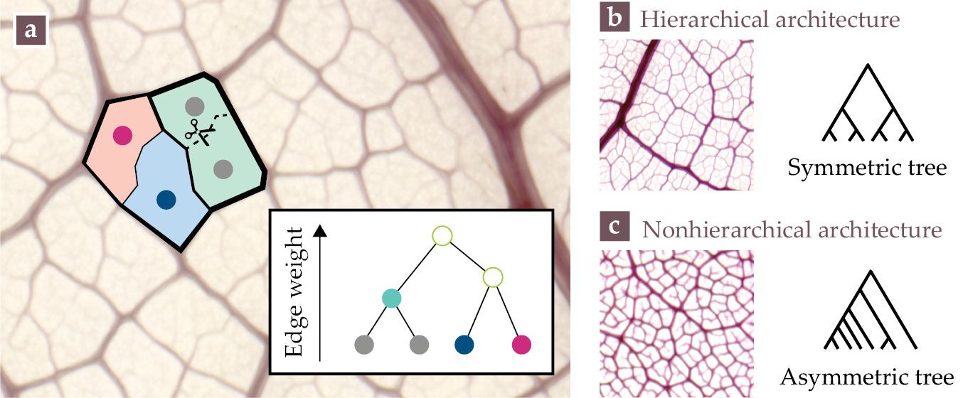
One starts by assigning a weight to each vascular segment, which is an edge between two junctions (that is, nodes) in a vascular network. Typical choices for edge weights are the segments’ radii or conductances. As sketched in figure 4a, one can use edge weight as a filtration parameter by sequentially removing edges, starting from the one with the smallest weight—that is, the least significant vascular segment—and then removing the others in order by weight until finally removing the edge with the largest weight. The key in the analysis is the order in which one removes the edges; the actual values of the edge weights are not important.

At each stage of the above hierarchical decomposition, one calculates quantities such as the aspect ratios of cycles and tracks how they evolve. One can thereby quantify how the cycles in a vascular network are related to each other. ¹⁴ Vascular networks range from highly nested, fractal-like structures (see figure 4b) to seemingly random structures that are not particularly hierarchical (see figure 4c). ¹⁵ The traits that one can examine using such a topological approach complement traits that carry information about edge widths, edge lengths, and network geometry. Studying topological and geometric features enables the algorithmic identification of leaf species from leaf fragments. ^{15 , 16} Such an approach to leaf identification is analogous to identifying people from their fingerprints.

The conductances of the edges in a network of flows, such as a vascular network, do not fully determine network function on their own. One also needs to know the boundary conditions of the flows and the sources that drive the flows. In the vascular system of an animal, for example, it is important to consider the location of the heart and how much blood it can pump. If one knows the boundary conditions and conductances of the edges in a network, one can calculate the pressure that drives the flow through each edge and the pressure drop along each edge. The pressure drops carry information about both network structure and network function, and they provide sufficient data to examine PH in a flow network. ¹⁷

Start, for instance, with an empty network and add edges one at a time in the order of the pressure differences along them. The pressure difference is thus a filtration parameter. Adjusting it yields a sequence of subnetworks of the original vascular network, and computing PH tracks topological changes across the sequence of subnetworks. For example, one knows which edge additions are birth edges that lead to the formation of new network components and which are death edges that merge existing components. A PD that records the births and deaths of components allows one to determine regions of the original vascular network that have relatively low pressure differences.

Think of a vascular network as a mountainous landscape in which the height of each edge is the pressure difference along that edge. If we start with an empty network, birth edges correspond to valleys (local minima) in the landscape and death edges correspond to the lowest mountain passes between neighboring valleys. If we instead start with a complete vascular network and remove edges one at a time, rather than adding them, then birth edges correspond to mountain peaks (local maxima) and death edges correspond to the highest mountain passes between neighboring peaks.

Rocks and colleagues used such a PH approach to study vascular networks that are tuned to deliver specific amounts of flow through particular edges or are tuned to have particular pressure drops along some predetermined edges. ¹⁷ They found well-delineated sectors of relatively uniform pressure that are not apparent from the underlying network structure. The pressure drops at the boundaries between those sectors revealed the pressures to which the networks were tuned.

Harnessing spatial features

Many of the examples that we have discussed are spatial in nature. A confounding factor in the use of PH to study spatial systems is that although it is able to capture information across different scales, traditional distance-based PH constructions can have trouble with applications in which differences in distance scales are less important than other features. For example, in human geographical data, traditional PH constructions often detect differences in population densities, like those between urban and rural areas. They can thereby miss important signals, such as voting patterns, that are not based on density.

Two of us (Feng and Porter) used PH to study spatial network models, street networks in cities, snowflakes, and spiderwebs. ¹⁸ We found it particularly amusing to examine the topological structure of webs that were built by spiders under the influence of psychotropic substances (see figure 5). The 2D images of spiderwebs provided initial surfaces for the construction of a filtered simplicial complex based on image geometry. The simplicial complex took advantage of the physical structure of spiderwebs and is also suitable for other images, maps, and so on. The topological structures of the spiderwebs—and, hence, the resulting PDs—differed considerably for spiders that were exposed to different drugs. The spiders that were given caffeine or chloral hydrate, a sedative used in sleeping pills, produced particularly abnormal webs.

Figure 5.

Outlook

Topological ideas have yielded many insights into the “shape” of data in diverse applications. However, many challenges remain. A key one is the incorporation of system features, such as spatial embeddedness and known physical properties, into the construction of simplicial complexes and thus into how one applies a topological lens. Topological approaches such as PH are enabling important advances in the study of physical phenomena, and they promise to yield further insights into condensed-matter systems, biophysical systems, and many other areas.

References

1. H. Edelsbrunner, J. L. Harer, Computational Topology: An Introduction, American Mathematical Society (2010).
2. G. Carlsson, Nat. Rev. Phys. 2, 697 (2020). https://doi.org/10.1038/s42254-020-00249-3
3. Q. H. Tran, M. Chen, Y. Hasegawa, Phys. Rev. E 103, 052127 (2021). https://doi.org/10.1103/PhysRevE.103.052127
4. P. Pranav et al., Astron. Astrophys. 627, A163 (2019). https://doi.org/10.1051/0004-6361/201834916
5. G. Yalnız, N. B. Budanur, Chaos 30, 033109 (2020). https://doi.org/10.1063/1.5122969
6. D. Leykam, D. G. Angelakis, https://arxiv.org/abs/2206.15075 .
7. N. Otter et al., EPJ Data Sci. 6, 17 (2017). https://doi.org/10.1140/epjds/s13688-017-0109-5
8. A. E. Sizemore et al., Netw. Neurosci. 3, 656 (2019). https://doi.org/10.1162/netn_a_00073
9. M. Feng et al., Front. Young Minds 9, 551557 (2021). https://doi.org/10.3389/frym.2021.551557
10. L. Papadopoulos et al., J. Complex Netw. 6, 485 (2018). https://doi.org/10.1093/comnet/cny005
11. L. Kondic et al., Europhys. Lett. 97, 54001 (2012). https://doi.org/10.1209/0295-5075/97/54001
12. J. W. Rocks, S. A. Ridout, A. J. Liu, APL Mater. 9, 021107 (2021). https://doi.org/10.1063/5.0035395
13. Y. Hiraoka et al., Proc. Natl. Acad. Sci. USA 113, 7035 (2016). https://doi.org/10.1073/pnas.1520877113
14. E. Katifori, M. O. Magnasco, PLoS One 7, e37994 (2012). https://doi.org/10.1371/journal.pone.0037994
15. H. Ronellenfitsch et al., PLoS Comput. Biol. 11, e1004680 (2015). https://doi.org/10.1371/journal.pcbi.1004680
16. B. Blonder et al., New Phytol. 228, 1796 (2020). https://doi.org/10.1111/nph.16830
17. J. W. Rocks, A. J. Liu, E. Katifori, Phys. Rev. Res. 2, 033234 (2020); https://doi.org/10.1103/PhysRevResearch.2.033234
J. W. Rocks, A. J. Liu, E. Katifori, Phys. Rev. Lett. 126, 028102 (2021). https://doi.org/10.1103/PhysRevLett.126.02810218. M. Feng, M. A. Porter, Phys. Rev. Res. 2, 033426 (2020). https://doi.org/10.1103/PhysRevResearch.2.033426
More about the authors
Mason A. Porter is a professor of mathematics at the University of California, Los Angeles and an external professor at the Santa Fe Institute in New Mexico. Michelle Feng is a postdoctoral scholar in computing and mathematical sciences at Caltech in Pasadena, California. Eleni Katifori is an associate professor of physics and astronomy at the University of Pennsylvania in Philadelphia.