The thinning of Arctic sea ice
DOI: 10.1063/1.3580491
During the first half of the 20th century, the Arctic sea-ice cover was thought to be in a near-steady seasonal cycle, reaching an area of roughly 15 million km2 each March and retreating to 7 million km2 each September. Ice thick enough to survive the melt season, termed perennial or multiyear ice (MYI), adds to the ice cover. A large fraction of MYI typically remained in the Arctic Basin for several years and grew to an equilibrium thickness of about 3.5 m—melting half a meter at the surface from June through August and growing by about half a meter at the bottom from October through March. In the late 1970s, MYI occupied more than two-thirds of the surface area of the Arctic Basin, with first-year ice (FYI) covering the remaining one-third. FYI is the thinner, seasonal ice that fills cracks in the ice cover and grows on the open ocean with the southward advance of the ice edge at the end of each summer.
That picture began to change significantly in the latter part of the century. Since 1979, passive microwave measurements by satellite, which can distinguish between the brightness signatures of ice and water, have established a more accurate account of the seasonal cycle of ice extent. The satellite record reveals that over the past 30 years the average September ice extent has been declining at an astonishing rate of more than 11% per decade (see figure 1 and the article by Josefino Comiso and Claire Parkinson in PHYSICS TODAY, August 2004, page 38 ).

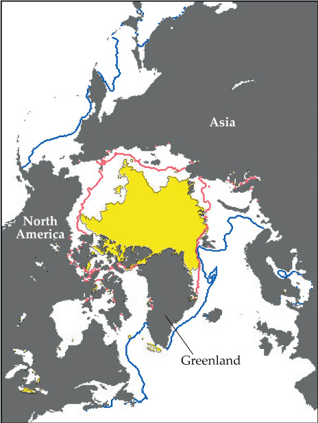
Figure 1. The extent of sea ice covering the Arctic Ocean expands and recedes seasonally. The median ice edges in March (blue) and in September (red) illustrate the extremes in area over the period 1979–2000. The yellow area shows the sea-ice extent at the end of summer 2010. (Data courtesy of the National Snow and Ice Data Center.)
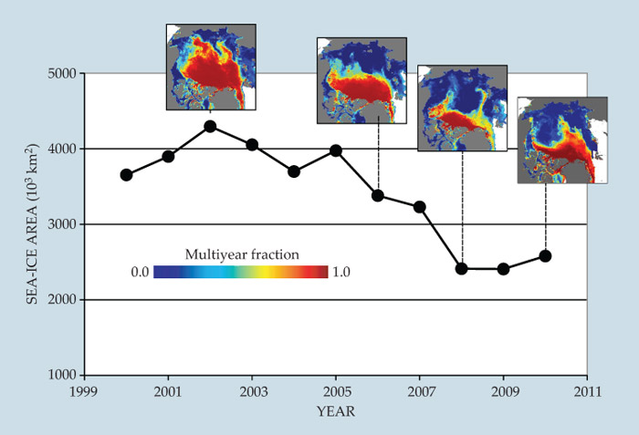
As a consequence, FYI has replaced much of the MYI in the Arctic Ocean. Satellite-borne radar scatterometers have made it possible during the past decade to identify and directly map the two primary ice types. As ice ages, brine drains from it, leaving air pockets behind; the older, less saline MYI is more than twice as reflective as seasonal ice. From that complementary satellite record, scientists witnessed a dramatic loss of MYI during the past decade, as illustrated in figure 2. Between 2004 and 2008, the winter cover of MYI shrank by 1.5 million km2—more than twice the size of Texas—and now covers only one-third of the Arctic Basin.

Figure 2. The decline of winter’s multiyear sea-ice coverage is evident from an analysis of data taken over the years 2000–10 by NASA’s Quick Scatterometer satellite and the European Space Agency’s Advanced Scatterometer satellite. The electromagnetic scattering properties of first-year ice and multiyear ice—that which survives more than one summer melt season—differ in salinity, surface roughness, and volume inclusions (that is, air pockets) that develop as sea ice ages. Those differences alter reflectivity and thus distinguish the two ice types in radar-backscatter measurements.
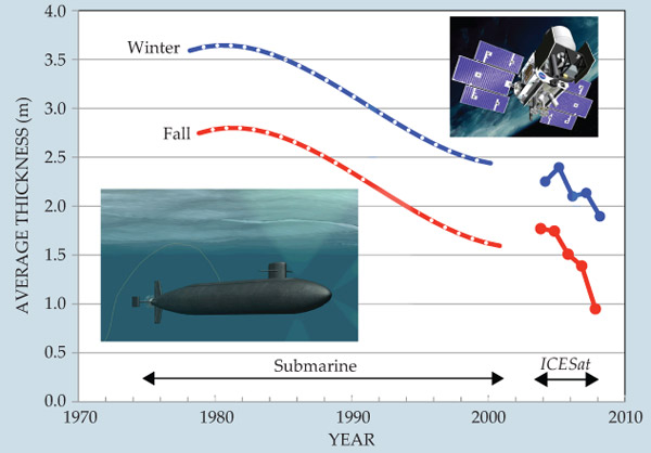
To determine the volume of melted sea ice and the associated changes in the heat lost or gained by the ice cover, one must make a basin-wide sampling not only of the ice’s area but also of its thickness. The latter is the technically more difficult measurement. Cross-Arctic estimates of thickness came with the first under-ice crossing of the Arctic Basin by the nuclear submarine USS Nautilus in 1958. Since the 1960s the US Navy has periodically declassified measurements of ice draft—the depth of the submerged portion of the floating ice observed by upward-looking sonars on submarines—for scientific analysis. The ice draft is converted to thickness using Archimedes’s principle and the densities of ice and seawater. Since 1979, researchers have been able to infer changes in the sea-ice thickness of the central Arctic using available submarine profiles. 1 The launch of the Ice, Cloud, and Land Elevation Satellite (ICESat) in 2003 made possible near-basin-scale mapping of ice thickness from space. The satellite’s light-detection-and-ranging (lidar) altimeter took readings of sea-ice freeboard—that part of the ice above the ocean surface—and thicknesses could then be deduced from those freeboard measurements just as they are from the ice draft.
The combined submarine and ICESat records, plotted in figure 3, show that the average sea-ice thickness of the central Arctic during winter has decreased from 3.5 m to less than 2 m over the past three decades. 2 Along with the observed decrease in sea-ice extent, there is a parallel thinning of the ice cover. If those rates persist, we are likely to eventually experience a seasonally ice-free Arctic Ocean (see PHYSICS TODAY, September 2009, page 19 ).

Figure 3. The thinning of the central Arctic sea-ice cover from 1978 to 2008 is evident from upward-looking sonar data recorded by US Navy submarines and by altimetry from NASA’s Ice, Cloud, and Land Elevation Satellite (ICESat), launched in 2003. The overall mean winter thickness of 3.64 m in 1980 can be compared with a 1.89-m mean during the last winter of the ICESat record—an astonishing decrease of 1.75 m in thickness. Between 1975 and 2000 the steepest rate of change was −0.08 m/yr in 1990. During ICESat’s recent five-year run through 2008, it recorded a still higher rate of −0.10 to −0.20 m/yr. (Adapted from ref. 2.)
That possibility has received increased public attention because the presence or absence of Arctic sea ice is a striking, important, and leading indicator of climate change. The shrinking ice cover has far-reaching consequences. Shifts in local climate affect marine ecosystems, endanger survival of birds and mammals, and pose a threat to the livelihood of indigenous communities around the Arctic Basin. Moreover, an ice-free ocean raises a plethora of issues concerning commercial shipping and resource extraction, all with long-term geopolitical and economic implications.
Changes in Arctic sea ice also influence deep convection in the marginal waters such as the Greenland and Labrador Seas. Those seas are sources of North Atlantic Deep Water, which contributes to the meridional overturning circulation (sometimes referred to as the conveyor belt), a global system of surface and deep currents that transports large amounts of water, heat, salt, carbon, nutrients, and other substances around the major oceans. That global circulation connects the ocean surface and atmosphere with the huge reservoir of the deep sea. Changes in the rate of production of North Atlantic Deep Water in the Arctic marginal seas have been shown to affect the Gulf Stream and hence climate, particularly that of Europe.
The observed rates of shrinking and thinning of sea ice in the Arctic Basin during the past three decades were greatly underestimated by the 2007 Intergovernmental Panel on Climate Change Fourth Assessment Report (IPCC–AR4) climate models; 3 indeed, none of the models can quantitatively explain the trends experienced in the Arctic. But the ice-free summers widely forecast in press reports as impending have not yet occurred. As long as some of the FYI is thick enough to survive the summer, and as long as the annual export of ice out of the Arctic Basin continues to be no more than the current annual average, a precipitous decline of the ice cover is not likely.
Thus the questions remain as to what actually caused the dramatic loss of ice and why the climate models have so underestimated its rate. Here we offer a perspective on the quality of the observational record, the gaps in our present understanding of the physical processes involved in maintaining and altering the sea ice.
Sea-ice dynamics
The dynamics of the ice cover is attributable to the wind and, to a lesser degree, the ocean currents. Due to the counterbalancing action of the atmospheric pressure gradients and the Coriolis effect, sea ice drifts roughly parallel to the frictionless wind above the surface, at about 1% of its speed. During winter, when the ice concentration—the fraction of the surface covered by ice—is near 100% and the mechanical strength of the ice is high, the surface stresses are propagated over distances comparable to the length scale of atmospheric weather systems. Fracture of the ice cover due to the gradients of the external stress results in the formation of ubiquitous welts of compressed ice blocks, known as pressure ridges, and openings in the ice caused by either diverging stresses or shear along jagged boundaries.
The approximate circulation pattern of sea ice has been known for more than a century, but it took the development of suitable satellite technology; automatic, drifting data buoys; and sophisticated methods of data transmission to develop a more detailed picture. Twenty institutions from nine different countries currently support the International Arctic Buoy Programme. Satellites have provided observations of ice motion on many different length scales. Generally, the circulation of sea ice is highly variable on weekly to monthly time scales but is dominated, on average, by a clockwise motion pattern in the western Arctic and by a persistent southward flow—the Transpolar Drift Stream—that exports approximately 10% of the area of the Arctic Basin through the Fram Strait every year. Figure 4a shows the average drift pattern and velocity of Arctic sea ice. An animation of the combined expression of the dynamic and thermodynamic processes—the drift of the ice and its seasonal expansion and regression during the years 1979–2009—is available at http://iabp.apl.washington.edu/data_movie.html .

Figure 4. Sea-ice circulation. (a) The two prominent features in the circulation of sea ice in the Arctic Ocean are the clockwise drift in the western Arctic’s Beaufort Gyre, which shoves sea ice against Greenland and the Canadian archipelago, and the Transpolar Drift Stream, which transports sea ice from the Siberian sector of the Arctic Basin out through the Fram Strait into the Greenland Sea. Ice drift is, on average, parallel to the atmospheric-pressure isobars (black lines). (b) The record of how much ice (blue) was annually transported through the Fram Strait between 1979 and 2008 correlates well with the atmospheric pressure gradient across the strait (red) at sea level. Every year about 10% of the Arctic Basin’s area is exported into the Greenland Sea. (Adapted from ref.
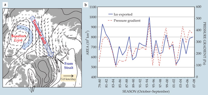
From a mass-balance perspective, the Arctic Ocean loses ice volume by melt and by export—hence the interest in southward transport of ice through the Fram Strait. The annual record of areal ice loss by export, based on satellite data of ice motion, can be seen in figure 4b. 4 Several authors have studied its anomalies and trends; remarkably, the data show no decadal trend. Much less can be said about a possible decadal trend in volume export—a more definitive measure of mass balance—due to the lack of an extended record of the thickness of ice floes that are exported through the Fram Strait. Although a recent study quite clearly shows that MYI loss in the Arctic Basin has occurred by melting during the past decade, 5 the relative contributions of melt and export to the loss remain uncertain.
Because of the system’s complexity, projections of sea-ice decline using global climate simulations are also problematic. Present-day sea-ice models include variations in the ice-thickness distributions that capture the interactions between dynamics and thermodynamics. 6 As ice thickens, it both becomes mechanically stronger and conducts less heat. The models compute ice velocities from the balance of forces acting on the ice: external stresses exerted by wind and ocean currents, and internal stresses that are due to the mechanical response of the ice cover. This response depends on the ice’s strength and thus its thickness distribution. During winter, the alternating diverging and converging motions of the ice cover modify the extremes of that distribution: Open water is exposed from cracks in some areas of the ice and pressure ridges develop in others. During summer, divergence of the ice controls the abundance of open water and alters the albedo feedback.
Projected September ice coverages from the global climate models used in the IPCC–AR4 range from ice-free conditions in September by 2060 to considerably more ice than is observed today. None of the models or their averages predict the trends of the past three decades. Although a majority of the global climate models include simulations of ice dynamics, proper interpretation of their results is confounded by uncertainties in the simulated atmospheric and oceanic forcing of the ice cover. For instance, two IPCC models with sophisticated ice dynamics and one with no ice-motion component all predict a near-zero September ice cover by 2060. With such discrepancies, it is difficult to identify the actual role of sea-ice dynamics in the projected ice behavior.
Thermodynamics
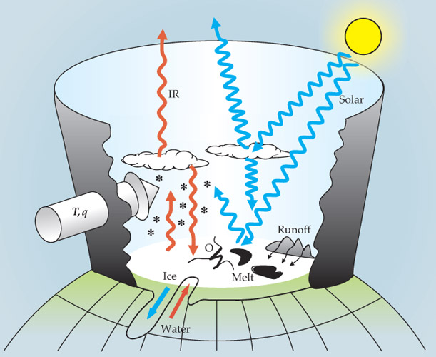
In the heat-energy balance, which describes the gain or loss of heat in the system, sketched in figure 5, the solar and atmospheric radiation terms dominate. Smaller in magnitude are the latent and sensible heat transported across the Arctic boundaries by atmospheric circulation and the sensible heat carried into the basin by the warm West Spitsbergen Current and by the Pacific inflow through the Bering Strait.

Figure 5. The heat and mass balance of the Arctic Basin. Incoming solar radiation (blue) is partially reflected, absorbed, and transmitted by clouds. The radiation reaching the surface is then partially reflected and absorbed in amounts that depend on the albedo of bare ice, open water (O), and numerous melt ponds formed during summer. River runoffs from surrounding continents feed the Arctic Ocean with fresh water. Infrared radiation (red) is emitted and absorbed by the clouds and the surface. Some of the atmospheric water vapor condenses and falls as snow, adding to the mass of the ice. The general circulation of the atmosphere results in a net influx of sensible and latent heat (T and q) from lower latitudes. The outflow of ice is primarily through the Fram Strait.
The surplus flux of thermodynamic energy needed to cause the observed thinning of the ice during the past half century is about 1 W/m2. (That flux is equivalent to a reduction in ice thickness of approximately 0.1 m/year.) In this section, we summarize the gaps in our understanding of the atmospheric and oceanic processes that are behind the surplus.
Ice–atmosphere interactions. Radiative energy fluxes from the atmosphere and the annual advection of sensible and latent energy from lower latitudes are two orders of magnitude larger than 1 W/m2. (Figure 5 illustrates those and other components of the mass and heat balance in the Arctic Basin.) At the moment, uncertainties in the heat-balance measurements observed at manned drifting stations and in the meridional heat transport calculated from radiosonde (balloon-based) observations around the Arctic perimeter prevent researchers from resolving those heat fluxes to an accuracy required to attribute the surplus of heat to any particular source or mechanism that explains the observed ice loss. 7
Ice–ocean heat storage. During summer, when the ice concentration is less than 100% and numerous melt ponds cover the ice, some fraction of the radiative energy is temporarily stored in the exposed water and delays the onset of freezing in autumn. In areas of low ice concentration and low albedo, the energy causes melting at the bottom and laterally around the perimeter of the ice floes. Recent observations 8 have found rates of ice-bottom melting as high as 1 m/month. Field observations of lateral melt are logistically difficult and laborious; repeated measurements of the same ice floe over the melt season are needed to characterize the process. The few reported measurements suggest that even thick ice floes can melt laterally up to several meters during summer,but the contribution of that process to the loss of MYI is not known.
One prospective approach for learning more about lateral melting is to mine the 1-m-resolution images collected by intelligence satellites—the so-called National Technical Means—and released to the public at http://gfl.usgs.gov . The fixed-location images acquired since the summer of 1999 reveal telling features of the ice surface. But studying the details of processes such as lateral melt will require sequential images of the same ensemble of ice floes to trace the history of surface changes during the melt season. Samples of such acquisitions have recently been released on the abovementioned website.
Ice–ocean heat flux. The rate of basal ice growth or melt is proportional to the difference between vertical heat conduction in the ice and turbulent heat flux in the ocean. One-dimensional thermodynamic ice models show that provided the surface energy balance is kept constant, the ocean heat flux derived from warmer-than-freezing water affects the equilibrium ice thickness most sensitively when the ice is thick. With that same constant-energy provision, an increase in the ocean heat flux from 1 to 2 W/m2 thins the equilibrium ice by 1 m/yr and an increase from 3 to 4 W/m2 thins it by only 0.5 m/yr. The heat carried into the Arctic Basin by the West Spitsbergen Current 9 and the Bering Strait inflow 10 has been documented by oceanographic moorings. But the mixing of those flows inside the Arctic Basin and the processes by which the imported warm water gives up its heat to the ice remain a subject of research. The only certainty is that a small change in ocean heat flux can have a large effect on ice thickness. 11
Snow and melt water
Owing to its low thermal conductivity, a blanket of snow slows the growth of underlying ice during the cold season. On the other hand, the onset of melting in early summer darkens the snow and, by albedo feedback, accelerates its own melting and that of the underlying ice. According to the thermodynamic model by Gary Maykut and one of us (Untersteiner), 12 an average snow depth of less than 1 m has little effect on the equilibrium ice thickness so long as, again, the energy balance at the surface is held constant. The less snow, the less time it takes to melt; the more the underlying ice melts, the thinner the ice is at the end of summer and the faster it grows during the following winter.
Over the Arctic Ocean, most of the snow falls in September and October. Thus new ice grown early in the season has the thickest snow cover. In contrast, calculations suggest, ice that starts to grow later in the cold of autumn or early winter in dynamically opened leads—areas of exposed water amid the pack ice—grows very quickly. That newly formed ice can thus overtake the older seasonal ice in thickness.
After the snow falls it is redistributed by the wind, which produces snow drifts behind pressure ridges; sweeps clean areas of flat, young ice; and blows snow into open leads. However, the clear and cold weather that usually follows a snowstorm induces a steep temperature gradient in the snow, which causes the snow to sublime and the vapor to diffuse upward toward surface layers. The process petrifies the snow within a day or two; rendered stiff, the snow remains in place for the balance of the winter. The overall impact of snow depth and its relationship to the underlying ice topography are not well understood, though.
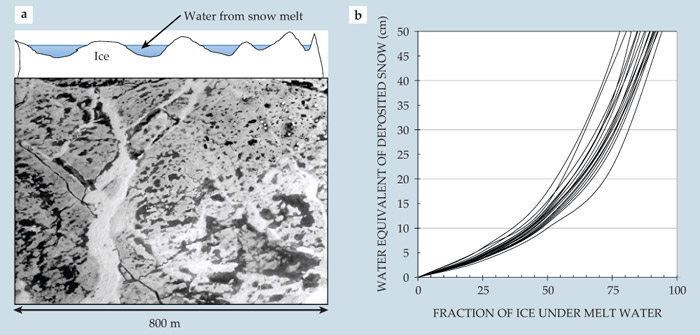
When the snow melts, however, melt-water ponds, which begin forming in June in the lowest or thinnest places on the surface, can exert a profound thermodynamic impact. The average snow cover on Arctic sea ice is about 33 cm, the equivalent of 11 cm of water, with an annual variability of 2 cm. 13 According to data shown in figure 6, an increase in the snow depth from 5 to 15 cm water equivalent would nearly double the area covered by ponds, where the melt rate is about 2.5 times that of bare ice. Given the variability in the spatial density of cracks and leads in different types of ice—thick, thin, young, old—it’s not known how far the melt water can travel over the surface to fill in the low places. There’s no doubt that surface topography and even small changes in available melt water substantially influence the ice loss during the melt season. But in the absence of measurements of surface relief and snow depth, it is difficult to quantitatively account for that influence.

Figure 6. (a) During summer, the Arctic Ocean’s ice is covered with residual patches of snow and melt ponds of variable depth and darkness—and thus variable albedo—as seen in this photograph from early July 1972; the white dots in the upper right are the huts of a research camp. Natural variations in surface topography create depressions that fill with water from snow melt during summer. (b) A 170-km elevation profile from an airborne laser altimeter taken northeast of Greenland—and parsed into 17 equal sections—shows the dependence of pond coverage on the amount of water available from snow melt. Even a modest increase in melt water can strongly influence the fraction of pond coverage and hence the surface albedo. (Data courtesy of Josefino Comiso.)
ICESat stopped taking data in 2009, and its successor, second-generation ICESat-2, is not scheduled to launch until early 2016. NASA’s IceBridge mission, the largest airborne survey of Earth’s polar ice cover ever flown, was launched in 2009 to fill the gap and ensure a continuous series of measurements. The hope is that high-resolution ice- and snow-depth profiles collected by the radars and lidars on IceBridge flights, along with imagery taken by reconnaissance National Technical Means satellites, may provide new insights into the problem. The European Space Agency’s ice mission known as CryoSat-2, launched last year, is also tasked with measuring changes in sea-ice thickness.
Outlook
As stated above, the net heat required to account for the average loss of ice during the past three decades is of similar magnitude to a 1-W/m2 global heat surplus. 14 Assuming that the surplus continues, and assuming that the global system does not undergo fundamental shifts, the share of heat received by the Arctic can be attributed to a host of variables and processes, including the cloudiness of Arctic skies; the distribution in the types of clouds; the temperature at the base of those clouds; changes in ocean-surface albedo; variations in the meridional transport of heat by the atmosphere, ice, and ocean; and the effect of greenhouse gases on all those factors. Gaps in our understanding of the processes that affect each factor represent a significant challenge to researchers attempting to assign specific causes for the thinning and loss of MYI or to project more detail than a general trend toward less Arctic ice in the future.
The loss of ice in the Arctic has made the region a crossroads of research, where the interests of science, environmental conservation and protection, resource development, and public policy meet. To produce useful ice forecasts that support societal needs, we see the following prospects.
On time scales of days to weeks, forecasting the state of the ice cover can be expected to proceed along traditional lines based mainly on meteorological methods and satellite observations. On time scales of years to decades, reliable projections face the problems of forecasting winds, cloudiness, surface albedo, and oceanic heat advection—all confounded by a plethora of climate-system feedbacks. Because sea ice is extremely sensitive to the least well-modeled and simulated part of the climate system—radiative heating from the clouds (see the article by Raymond T. Pierrehumbert in PHYSICS TODAY, January 2011, page 33 )—it seems difficult to predict more than the fact that Arctic sea ice is likely to diminish.
Year-round field programs and repeated airborne surveys by aircraft are operationally limited and expensive. The best prospects for supporting and improving seasonal ice prediction may well come from initializing model ensembles with the most current atmospheric, ocean, and ice analyses. Input to those analyses would come from satellite surveys capable of providing near real-time observations of key ice, ocean, and atmospheric parameters. Instead of the project-based, sporadic deployments of oceanographic moorings now common, a sustained international program to deploy and maintain such instruments at strategic locations will be especially useful.
Perhaps equally useful as a predictive tool for long-term behavior are simplified, low-order models of the physical processes described in this article. Those models may provide insight regarding quantitative changes one might expect on multiple time scales.
Satellite altimetry and imagery used to track the changes of ice properties within ice parcels on the scale of a meter will remain crucial for understanding the physical processes that control the Arctic’s evolution, particularly when the observations are supplemented with occasional short-term field studies. We believe that a greater degree of coordination between those field studies and the use of civilian and intelligence satellites is essential.
We thank John Wettlaufer, Ian Eisenman, and Steve Warren for their careful reading and constructive criticism of the manuscript.
References
1. D. A. Rothrock, D. B. Percival, M. Wensnahan, J. Geophys. Res. https://doi.org/JGREA2 https://doi.org/JGREA2 113, C05003 (2008),
10.1029/2007JC004252 .2. R. Kwok, D. A. Rothrock, Geophys. Res. Lett. https://doi.org/GPRLAJ 36, L15501 (2009),
10.1029/2009GL039035 .3. J. Stroeve, et al. Geophys. Res. Lett. https://doi.org/GPRLAJ 34, L09501 (2007),
10.1029/2007GL029703 .4. R. Kwok, J. Clim., 22, 2438 (2009),https://doi.org/10.1175/2008JCLI2819.1 .
5. R. Kwok, G. F. Cunningham, Geophys. Res. Lett. https://doi.org/GPRLAJ 37, L20501 (2010),
10.1029/2010GL044678 .6. A. S. Thorndike, J. Geophys. Res. https://doi.org/JGREA2 https://doi.org/JGREA2 97, 9401 (1992),
10.1029/92JC00695 .7. For an examination of the Arctic’s large-scale energy budget compared with reanalysis by the National Centers for Environmental Prediction and the National Center for Atmospheric Research, see M. C. Serreze, et al. J. Geophys. Res. https://doi.org/JGREA2 https://doi.org/JGREA2 112, D11122 (2007),
10.1029/2006JD008230 .8. D. K. Perovich, et al. J. Geophys. Res. https://doi.org/JGREA2 https://doi.org/JGREA2 108, 8050 (2003),
10.1029/2001JC001079 .9. E. Fahrbach, et al. Polar Res. 20, 217 (2001).
10. R. A. Woodgate, T. Weingartner, R. Lindsay, Geophys. Res. Lett. https://doi.org/GPRLAJ 37, L01602 (2010),
10.1029/2009GL041621 .11. I. V. Polyakov et al. J. Phys. Oceanogr. https://doi.org/JPYOBT 40, 2743 (2010).
12. G. A. Maykut, N. Untersteiner, J. Geophys. Res. https://doi.org/JGREA2 https://doi.org/JGREA2 76, 1550 (1971),
10.1029/JC076i006p01550 .13. S. G. Warren, et al. J. Clim. 12, 1814 (1999).
14. K. E. Trenberth , Curr. Opin. Environ. Sustain. 1, 19 (2009).
More about the authors
Ron Kwok is a senior research scientist at the Jet Propulsion Laboratory, California Institute of Technology, in Pasadena. Norbert Untersteiner is an emeritus professor of atmospheric sciences and geophysics at the University of Washington in Seattle.


