The math behind the scene of the crime

Under the soft hum of sodium street lamps, a shadowy figure prowls the nighttime street. As he approaches a car parked between the cones of light cast down by the lamps above, he pauses, then reaches into his jacket. The near silence of the night is split by the unmistakable crackling of breaking glass; the car’s side window lies shattered on the sidewalk. The figure, working quickly, reaches inside the vehicle and grabs the backpack that the car’s owner left under the passenger’s seat. It looks to be another easy score. But suddenly, the thief’s world is bathed in pulsing blue light, and his ears ache with the piercing wail of a police siren. “Freeze,” commands the police officer, who has been lying in wait for just such an occasion and was guided to this location by his new partner, a computer program.

Could crimes really be predicted by a computer? My colleagues and I think so, and we have spent the past several years developing mathematical theories that not only aim to explain patterns in crime but also help to predict where and when crimes would be likely to occur in the near future.

Little boxes

Unless you are one of the few who own items of exquisite value—unique works of art, rare jewelry, and such—your home is unlikely to be cased by a burglar. Rather, if you are burgled, your home was probably just in the wrong place at the wrong time. That is to say, your home was somewhere along your burglar’s daily route, and the burglary was a crime of opportunity.

Unfortunately for those of you who have had your homes burgled, criminals tend to return to homes they have hit previously (repeat victimization) or to neighboring homes (near-repeat victimization). After all, having stolen from you once, the burglar has much more information about your home than almost any other; he knows what types of goods are present, what forms of security protect it, and when the occupants are not home. So returning to your home minimizes uncertainty and the risk of being caught. And since nearby homes and their occupants are often similar in many regards, your burglar may feel more comfortable burgling one of your neighbor’s homes, which are also along his daily route, than he would hitting a home on the opposite side of the city. Furthermore, even if your burglar himself does not return, the original incident may have left a physical mark on your house, such as a broken window, that perhaps subconsciously indicates to other potential criminals that your home is not well guarded and might be an easy target.

The tendency of criminals to revisit the same locations repeatedly leads to areas of elevated crime risk. Mapping those hot spots as they arise is one technique that police agencies have used to fight crime. It is not clear, however, how to best construct such hot-spot maps. Moreover, the police would really like to make a prospective map of tomorrow’s hot spots before the crimes have been committed. To address those issues, my colleagues and I turned to mathematics. Our goal was to construct a relatively simple model that describes the formation and dynamics of certain classes of crime hot spots, given the criminal psychology discussed above.

Criminal attraction

We realized our model for crime hot spots first as an agent-based simulation—a computer program that simulates many essentially identical criminal agents as they go about their daily routines within a virtual city and occasionally commit crimes. At each location within the city, agents are randomly generated at a specified rate Γ. Once they are virtually born, they move throughout the city looking for crime opportunities. The decision of a criminal agent to commit a crime at a given location i in the city is made probabilistically, with the instantaneous rate of crimes at the location called the attractiveness, A_i.

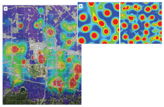
If the criminal does not commit a crime at his current location, then he will move to an adjacent location in the city by executing a biased random walk. That is, he chooses to move to a neighboring location j with a probability that is directly proportional to A_j. As a result, the criminal tends to move to areas of the city that he finds more attractive for crimes. We reasoned that on any given outing, a criminal would only commit one crime. So whenever a criminal does commit a crime, the algorithm removes him from the city—think of that removal as representing the criminal heading home with his loot, to return again to active status at some random time determined by the birth rate Γ. As described so far, the simulation captures the opportunistic nature of most crimes in a simple manner.

To model repeat victimization requires a bit more work. We supposed that the attractiveness of a location i is a linear combination of two factors: an intrinsic attractiveness, A⁰, constant in space and time, and a dynamic attractiveness, B_i, which varies in time as crimes are (or aren’t) committed nearby. (In the real world, the intrinsic attractiveness probably depends on position. But let’s keep it simple.) Specifically, whenever a crime occurs at location i, B_i increases by some specified amount ϴ. As a result, crimes are more likely to take place there in the future. To allow for near-repeat victimization, at each round of the simulation we take a fraction η of the dynamic attractiveness at i and spread it among its neighbors. Thus locations near crime sites become more likely spots for crimes as well. But to limit those effects to only the near future, we also force B_i to decay exponentially over time, with a decay rate ω.

The agent-based model just described contains several parameters that affect the behavior of a simulation; some parameter values lead to crime hot spots, and others don’t. Unfortunately, it is difficult to predict how the values of any of the model’s individual parameters will change the results of the simulation, so we faced the discomforting proposition of having to run the simulation thousands of times with varying parameters to determine how each one affects the outcome. But at least for big cities with many criminals, there is another way. We can appeal to the law of large numbers and use expectation values of probabilistic events. The result of that appeal is a much simplified form of the model, which may be written as two coupled partial differential equations:

Here A describes local attractiveness and ρ describes a density of criminals. The remaining three parameters are dimensionless. The spreading parameter η has the same interpretation as in the agent-based simulation; A⁰ is a scaled version of the intrinsic attractiveness from the agent-based model; and A‾, the spatial average of A in the steady state, is built from the other parameters of the simulation.

With the above system of equations in hand, we could answer a variety of previously daunting questions about crime hot spots. One particularly interesting finding is governed by the inequality

Though far from obvious, satisfying the inequality basically means that crimes are close enough that their near-repeat regions may overlap and begin to form hot spots, but not so close that the hot spots glom into one giant crime nightmare. We give the name supercritical to those hot spots formed when the inequality is satisfied to distinguish them from other types—subcritical hot spots—that can develop if the inequality is not satisfied, provided there is a very large concentration of crime in an area to begin with. The two types respond very differently to police intervention, which we model by temporarily setting the local attractiveness within existing hot spots equal to zero: Supercritical hot spots merely shift to locations that the police are not suppressing, but subcritical ones can be eradicated if the police presence is sufficient.

Our theory has shed light on the conditions under which crime hot spots form and on their dynamics and responses to police intervention. Inspired by what we have learned, we have developed further techniques tailored to the task of computing prospective maps based on past criminal activity. The tools we have developed are now in use by several police departments internationally, and the once fantastical idea of computer programs predicting crime in advance is slowly becoming reality.

References

1. J. Q. Wilson, G. L. Kelling, “Broken windows: The police and neighborhood safety,” Atlantic Monthly 249(3), 29 (1982).
2. M. B. Short et al., “A statistical model of criminal behavior,” Math. Models Methods Appl. Sci. 18(suppl.), 1249 (2008).
3. M. B. Short et al., “Dissipation and displacement of hotspots in reaction-diffusion models of crime,” Proc. Natl. Acad. Sci. USA 107, 3961 (2010).
4. M. B. Short, A. L. Bertozzi, P. J. Brantingham, “Nonlinear patterns in urban crime: Hotspots, bifurcations, and suppression,” SIAM J. Appl. Dyn. Syst. 9, 462 (2010).
5. G. O. Mohler et al., “Self-exciting point process modeling of crime,” J. Am. Stat. Assoc. 106, 100 (2011).
More about the authors
Martin Short is an assistant professor of mathematics at the Georgia Institute of Technology in Atlanta.