The Unusual Thermodynamics of Microscopic Systems

The thermodynamic behavior of microscopic systems can be quite different from that of macroscopic systems, for which fluctuations in thermodynamic quantities are usually negligible. As physicists strive to build ever smaller machines, it becomes important to understand, for example, the statistics of the work done on or by a machine as it moves from an initial to a final state. That work is not simply a function of the beginning and ending states. But—according to the usual telling of the story—the work is determined once one is given a path or process that connects the states.

The usual story is not strictly accurate. For example, in a system connected to a heat bath, uncertainties of order kT arise from the Boltzmann distribution of energies in the initial and final states, and also from energy exchange with the heat bath as the system moves along a path connecting those states. That means the work given to a system cannot be uniquely specified, even if the path is known. The energy uncertainties in macroscopic systems, though, are tiny compared to the average work. Thus, for practical purposes, one can say that two states and a connecting path determine work in those systems. If the system is microscopic, the statistical distribution of work associated with the system’s change from its initial to its final state can have practical consequences.

Over the past decade, a good deal of theoretical effort has been devoted to spelling out the nature of work distributions. In the past few months, experimental tests have been conducted for two particular theoretical results—the transient fluctuation theorem of Denis Evans (Australian National University in Canberra) and Debra Searles (Griffith University in Brisbane) ¹ and the nonequilibrium work relation derived by Chris Jarzynski (now at Los Alamos National Lab) ² .

Evans and Searles joined forces with three other colleagues from ANU to test the transient fluctuation theorem. ³ At about the same time, a team from the University of California, Berkeley, and Lawrence Berkeley National Laboratory, led by Carlos Bustamante, explored the validity of the nonequilibrium work relation. ⁴ Both theoretical predictions passed admirably.

Transient fluctuation theorem

The transient fluctuation theorem is one of many that tackle the statistical nature of fluctuations. Specific forms of the various theorems depend on which thermodynamic parameters (temperature, volume, and so forth) are held constant, whether the system is prepared in an equilibrium state, and other factors. The transient fluctuation theorem tested by Evans and coworkers applies to systems in a constant-temperature environment and initially at equilibrium. For the Australian team’s work, in which an optical trap interacts with an experimental vessel, the theorem assumes the form $$P\left(W\right)/P\left(-W\right)=exp\left(W\right).$$

Here, W is a dimensionless number giving the work (divided by kT) delivered to the vessel; P(W) is the probability that, in a given experiment, work W will be delivered to the vessel; and P(—W) is the probability that the vessel does work W on the trap. Multiplying both sides of the above equation by P(–W) and integrating over W from – ∞ to 0 yields an integrated version of the fluctuation theorem $${P\left(W<0\right)/P\left(W>0\right)=〈exp\left(-W\right)〉}_{+},$$ where P(W < 0) is the probability that the vessel does work on the trap and P(W > 0) is the probability that the trap does work on the vessel. The angle brackets and subscript denote an average over all trajectories with positive work delivered to the vessel.

Testing transient fluctuations

To test the transient fluctuation theorem, Evans and colleagues measured the work delivered to a room-temperature vessel consisting of 6.3 μm-diameter latex beads in contact with a water bath. A focused external laser beam created an optical trap that exerts a Hooke’s-law restoring force with known force constant on a bead near its focal point. Initially the vessel was at rest and a bead was allowed to come to equilibrium in the trap. Then Evans and coworkers moved the vessel at 1.25 μm/s relative to the fixed trap. As a consequence of this movement, the bead was dragged away from the focus of the trap and subject to an external force, which causes it to move in the trap’s potential well.

The Australian group observed the latex bead’s position 100 times per second for a total of 10 seconds. At each time step, the position of the bead yielded the force exerted by the optical trap. The product of force and the distance the vessel moved gave the incremental work added to the vessel by the trap at each time step. Effects associated with the initial acceleration of the vessel were negligible.

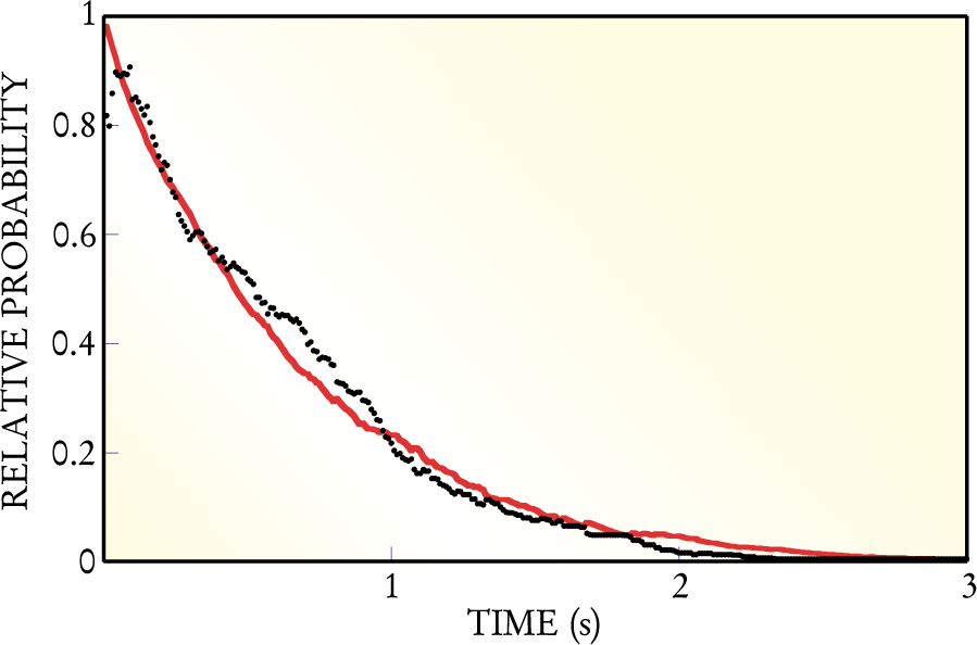
Figure 1 shows the experimentally determined values for the right- and left-hand sides of the integrated fluctuation theorem as a function of time for the 540 trajectories studied by the Australian group. The two curves agree to within statistical error. Discrepancies at early times, for which the work values are small, may arise because of experimental limitations in measuring the position of the bead and difficulty in determining the precise time at which the vessel began to move.

The nonzero probability for negative work observed for up to about two seconds is worthy of comment. Imagine, as is often the case, that after a certain time, the bead has a higher energy than it had initially. Then, if the work done by the trap on the vessel (bead plus bath) is negative, energy has been delivered to both the bead and the optical trap interacting with the vessel. That energy came from the water bath—just the sort of energy transfer prohibited by the second law in the thermodynamic limit of infinitely large systems: Heat has been converted to work with 100% efficiency.

Nonequilibrium work relation

Bustamante and his colleagues measured the work delivered as they stretched and recompressed a folded RNA molecule that was prepared in equilibrium and kept in a constant-temperature and constant-pressure environment. Associated with the change in length of the molecule is a change in the Gibbs free energy, which can be thought of as the work needed to reversibly change the length. (For reversible processes, the work is well defined.) When one manipulates a system so as to change its free energy, a generalized form of the transient fluctuation theorem reflects that change: ⁵ $$P\left(W\right)/P_R\left(-W\right)=exp\left(W-\Delta G\right).$$

Here, P _R denotes the probability distribution for the process that is the time reversal of the “forward” process yielding the distribution P, and ΔG is the change in the free energy (divided by kT). So, for example, in the Berkeley experiment, if the forward process is stretching the RNA molecule, the reverse process is compressing it. In the Australian experiment, time reversal takes a right-moving vessel and gives it a velocity to the left. Left–right symmetry means that for that experiment, one need not distinguish between the forward and time-reversed distributions.

Multiply both sides of the preceding equation by P _R(–W)exp(–W) and integrate over W from –∞ to +∞. Because G is a state function, its change comes out of the work integral, and yields the result $$exp\left(-\Delta G\right)=〈exp\left(-W\right)〉,$$ where the angle brackets denote an average over all trials. The remarkable feature of this so-called nonequilibrium work relation is that it allows extraction of information about a system’s free energy change—a property of its equilibrium states—by studying the work distribution arising from a series of processes in which the system starts at equilibrium but need not be in equilibrium at any other time (including in its final state). Jarzynski derived the nonequilibrium work relation from first principles in 1997. The later elegant demonstration beginning from the generalized transient fluctuation theorem is due to Berkeley’s Gavin Crooks. ⁵

Testing nonequilibrium work

If one stretches a rubber band very slowly, and then lets it slowly relax, one does no net work on the band. But if the rubber band is stretched quickly, its force constant increases. Quick compression yields a reduced force constant. For rapid operation, one does net work on the band even though its final and initial states are the same.

The folded RNA molecule that Bustamante and colleagues studied is similar to the rubber band in many respects. When the Berkeley group unfolded and refolded the molecule slowly enough, increasing the applied force, say, by 5 piconewtons each second, the process was essentially reversible: In particular, to within experimental error, no net work was associated with an unfolding–refolding cycle. When they unfolded and refolded the RNA rapidly (34 and 52 pN/s) they generally did work on the molecule. But the transient fluctuation theorem asserts, and Bustamante and colleagues confirmed, that sometimes the work was negative.

To manipulate the RNA molecule, the Berkeley group attached each end of the RNA molecule to its own polystyrene bead. One bead was deliberately moved a measured distance, which stretched the RNA molecule, while the other was held in an optical trap (but also moved in response to the stretching). The Berkeley group determined the force acting on the RNA molecule by measuring the deflection of the trapping laser beams. From that force, they deduced the position of the bead in the trap.

By stretching the RNA molecule slowly and measuring the work input, the Berkeley group determined the molecule’s free energy as a function of the amount by which it was stretched. Two different rates of rapid stretching then yielded two different (extension-dependent) work distributions that were plugged into the nonequilibrium work relation to estimate the free energy as a function of extension.

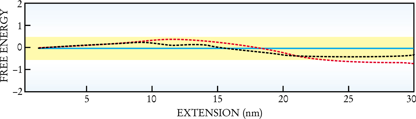
Figure 2 shows the difference between the free energies calculated from Jarzynski’s relation and the free energy measured in experiments conducted slowly enough to approximate them as reversible. Except for the fastest stretching rate and the greatest extensions, the two agree within experimental error, confirming the nonequilibrium work relation.

Systematic errors might account for the discrepancies. Because of the exponential averaging in Jarzynski’s result, the nonequilibrium work relation strongly weights those runs for which the work is less than the free-energy change. Therefore, instrument noise tends to lead to an underestimate of the free energy, especially for large extensions, since noise piles up over the time needed to produce such extensions.

Figure 2 does not present error bars for the estimates based on the nonequilibrium work relation. For the non-Gaussian distributions involved, conventional error analysis can be misleading. One possible estimate, based on the standard error of the mean, gives relatively small errors. ⁴

Clunky small machines

A consequence of the transient fluctuation theorem is that microscopic machines will work differently from their macroscopic counterparts. If an engine is made small enough so that the work performed during a cycle is comparable to kT, then occasionally and uncontrollably it will not run as designed. Imagining a tiny car with a tiny engine, Evans observes that the car won’t run straight down the interstate but will jump “two steps forward, one step back.” You’ll get to where you want to go, but the ride won’t be smooth. “The bottom line,” comments Jarzynski, “is that we’re starting to understand more quantitatively the nature of thermodynamic fluctuations at the microscopic level.”

References

1. D. J. Evans, D. J. Searles, Phys. Rev. E 50, 1645 (1994).https://doi.org/10.1103/PhysRevE.50.1645
2. C. Jarzynski, Phys. Rev. Lett. 78, 2690 (1997).https://doi.org/10.1103/PhysRevLett.78.2690
3. G. M. Wang et al., Phys. Rev. Lett. 89, 050601 (2002).https://doi.org/10.1103/PhysRevLett.89.050601
4. J. Liphardt et al., Science 296, 1832 (2002).https://doi.org/10.1126/science.1071152
5. G. E. Crooks, Phys. Rev. E 60, 2721 (1999).https://doi.org/10.1103/PhysRevE.60.2721