Random walkers illuminate a math problem

In a 1905 issue of Nature, statistician Karl Pearson of University College London asked readers for their help with a problem he named the random walk ¹ : A walker starts at an origin point and walks l yards in a straight line in a random direction. The walker then turns and proceeds another l yards in another random direction, and the process repeats n times. Having found the solution only for the case of two steps, Pearson wanted an expression for the probability that the walker is a radius r from the starting point after n steps.

In the intervening 114 years, the random walk—or, more colorfully, the drunkard’s walk—has been applied to such diverse fields as ecology, economics, computer science, biology, chemistry, and physics, and it helped produce the art on the cover of this issue. Physicists use the random walk to model diffusion, Brownian motion, polymers, and even quantum field theory. Random walkers can move in one, two, or more dimensions, and their steps can have a fixed length or a probabilistic distribution of possible lengths. Figure 1 is an example of a simulated two-dimensional random walk with a fixed step length.

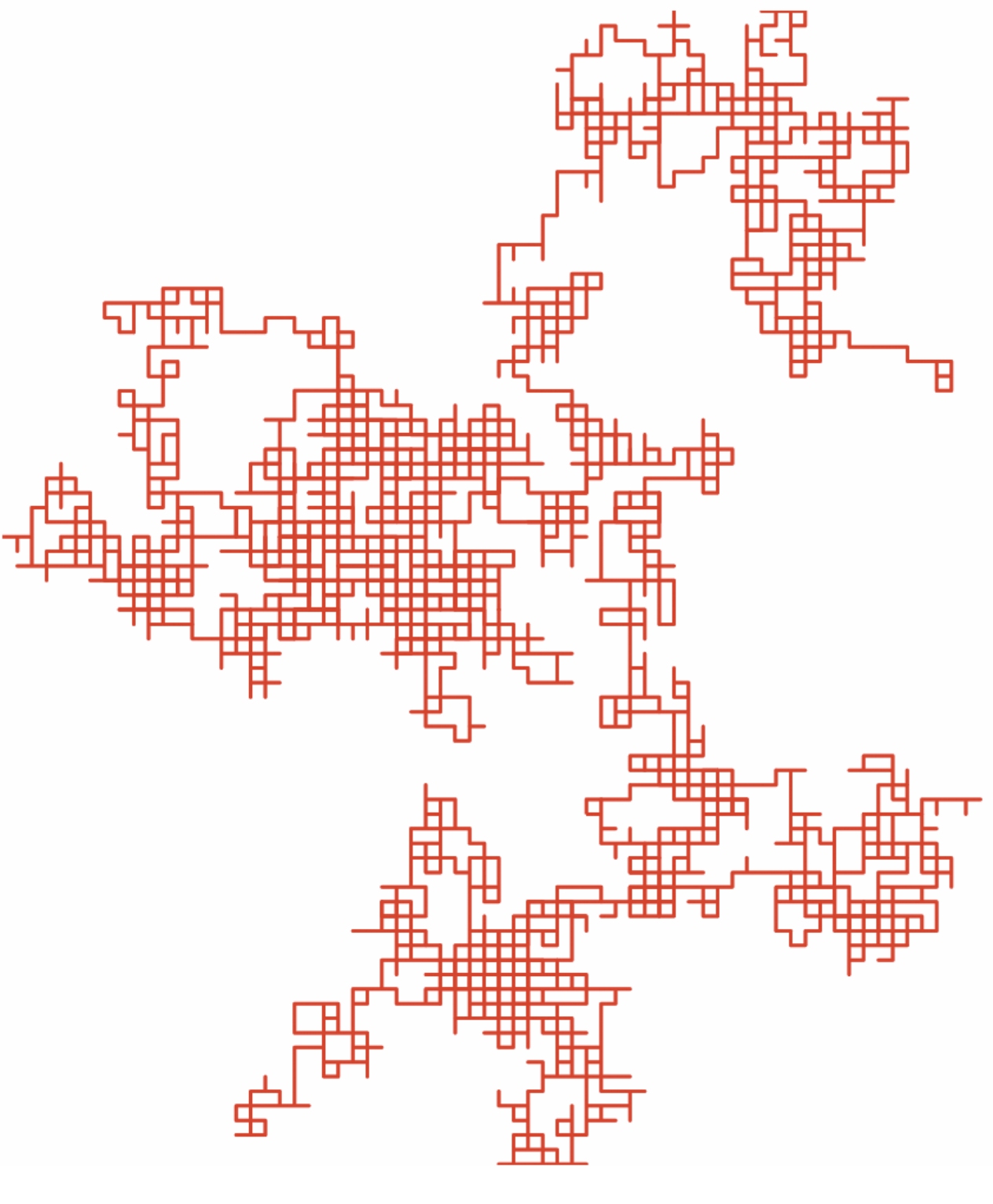
Figure 1.

Random walks can now add solving integrals to their resume because of the work of Satya Majumdar and Emmanuel Trizac of Université Paris–Sud/CNRS. ² The project started one Sunday in May 2018 when a Twitter post captured their attention. The tweet, from Fermat’s Library (@fermatslibrary ), presented a mathematical oddity: A family of successively larger integrals follows an apparent pattern that breaks down unexpectedly without an intuitive mathematical explanation. But when the integrals are framed as random walks, all becomes clear.

Integral to our understanding

The integrals I_n in question are shown in figure 2. They are one variant of Borwein integrals, which integrate over products of sin(a_nx)/a_nx factors; the a_n coefficients take a different value for each factor and for each variant. The integral I₁ with only the n = 1 factor is π. The integral I₂ with two factors, I₃ with three factors, and even up to I₇ with seven factors are also all π. But the integral I₈ with eight factors is short of π by less than 10⁻¹⁰. That odd behavior was first reported in 2001 by David Borwein of the University of Western Ontario and his son Jonathan Borwein of Simon Fraser University. ³ Numerical calculations uncovered the deviation, which, because it was both small and unexpected, was first attributed to a software bug. But it wasn’t a bug; it was a behavior found in all variants of the sin(a_nx)/a_nx integrals, now named after the two researchers, and in many related integrals with additional functions in the integrand.

Figure 2.

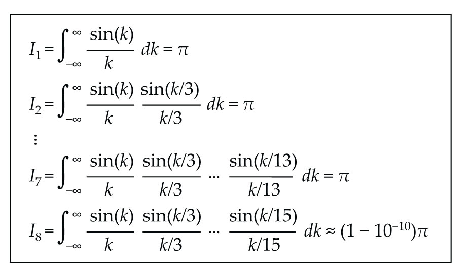
The Borweins found an expression for the first integral that deviates from the pattern in all Borwein integrals. If the first coefficient a₁ is larger than the sum a₂ + … + a_j of all the rest of the coefficients, the integral gives the expected value. In I₃, for example, the coefficients are 1, ⅓, and ⅕; 1 > ⅓ + ⅕, and the integral is π, as expected. Once the sum exceeds the first coefficient, the value of the integral changes. For the integrals in figure 2, that transition first happens for I₈, which is less than π. But mathematicians have lacked an intuitive understanding of why the change happens.

Inspired by the tweet, Majumdar and Trizac hoped a physics perspective might offer some insight to the problem, and they began searching for a relevant reformulation. The pattern breaking reminded the pair of a phase change, but the resemblance proved fruitless. It was then that the structure of the integral reminded them of a Fourier transform. With that insight, the connection to random walkers became obvious.

Walk the line

Majumdar and Trizac restricted their imagined random walkers to a 1D walk with the ability to share the same position. They started with an infinite number of random walkers spread out evenly along an infinitely long line. When all the walkers take random steps, the number of walkers that leave a position—call it position x = 0—is the same as the number of walkers that land on that same position. No matter how many steps the random walkers take, the total number at x = 0 stays the same.

But what if the random walkers occupy a finite space? If they start from x = 0 and take an initial step with a size equally distributed in the range |Δx| ≤ 1, the walkers will be evenly spread from −1 to 1 (see the left panel of figure 3), and the Fourier transform of that rectangular distribution is sin(k)/k in terms of the conjugate variable k. The first Borwein integral in figure 2 can be reimagined as the Fourier transform of sin(k)/k evaluated at x = 0, or the density of random walkers at the origin. For those walkers at x = 0, the initial distribution looks the same as the case with walkers spread to infinity.

Figure 3.

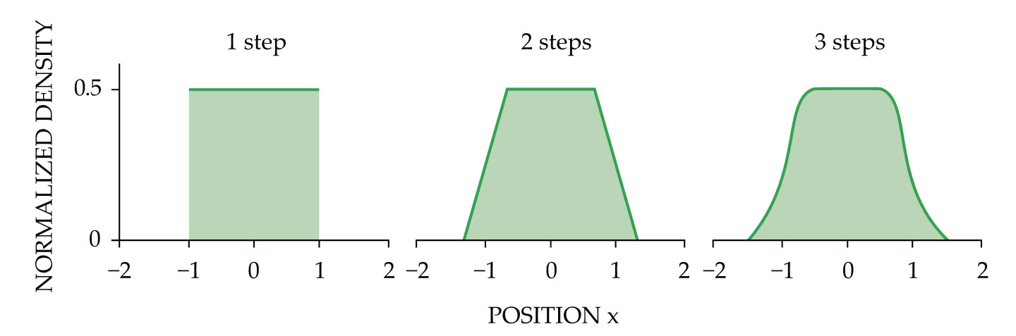
The second integral calculates the fraction of walkers at x = 0 after they each take a second step with |Δx| ≤ ⅓. Another step with |Δx| ≤ ⅕ produces the situation in the third integral, and so on. With each step, the random walkers spread out more (see the middle and right panels of figure 3) and look less like the infinite case, but it takes eight steps for the number of walkers at the origin—and thus the Borwein integral—to change. That’s because the density at x = 0 stays the same as the infinite case until the information that initially there were no walkers beyond ±1 reaches the origin. A random walker starting at x = −1 and acting as a messenger travels at most ⅓ + ⅕ + … + 1/(2j−1) after j steps. The walker gets to the origin only after the eighth (1/15) step. That argument, based on the rate at which information propagates, is equivalent to the Borweins’ expression, but Majumdar and Trizac show why it’s correct.

Their intuitive picture does more than reveal when the results of the integrals change; it also offers a way to avoid directly calculating those complicated integrals. One simply finds the normalized density of random walkers at x = 0. The density after the first step—and the next six steps—is ½, which needs to be multiplied by a factor of 2π to get the value of the first seven integrals. That calculation-free route to the solution will be important for other integrals that haven’t been or can’t easily be numerically solved.

All in the family

The method from Majumdar and Trizac applies to all variants of Borwein and many similar integrals. One such family of integrals takes the form of those in figure 2, with the addition of a cos(k) factor in the integrand. With a similar Fourier transform reimagining, the integrals still represent the density of random walkers, but now at x = 1. The random walkers at at that position know that there are no walkers beyond x = 1. But they are unaware that there are no walkers below −1. Thus they behave the same as if the walkers stretched infinitely far, until the information from x = −1 reaches them—that is, when the steps add up to 2. That happens at the 57th step, which is when the value of the integral decreases by 10⁻¹¹⁰.

The same logic can be applied for families of integrals in which the walkers start evenly distributed in a finite range or all the walkers start at two points ±b, as defined by a coefficient b in a cosine or Bessel function. The walkers can take steps with a range of sizes, as defined by the coefficients a_n in sin(a_nx)/a_nx factors, or any other distribution of steps as long as they are bounded. And if no longer confined to 1D, random walkers can be applied to integrals in any number of dimensions. “We have put forward a tool that hopefully will prove useful for computing even more complex quantities,” says Trizac.

In addition to their purely mathematical interest, sin(ax)/ax functions and integrals of those functions appear frequently, perhaps unsurprisingly, in Fourier analysis—for example, the sin(ax)/ax function is used to smooth Fourier series. Fields such as acoustics and optics rely heavily on Fourier analysis for signal processing. But the connection with random walkers may open up new avenues for applications.

References

1. K. Pearson, Nature 72, 294 (1905). https://doi.org/10.1038/072294b0
2. S. N. Majumdar, E. Trizac, Phys. Rev. Lett. 123, 020201 (2019). https://doi.org/10.1103/PhysRevLett.123.020201
3. D. Borwein, J. M. Borwein, Ramanujan J. 5, 73 (2001). https://doi.org/10.1023/A:1011497229317