Quantum Shot Noise
DOI: 10.1063/1.1583532
“The noise is the signal” was a saying of Rolf Landauer, one of the founding fathers of mesoscopic physics. What he meant was that fluctuations in time of a measurement can be a source of information that is not present in the time-averaged value. As figure 1 reminds us, some types of noise are more interesting than others. A physicist with access to sensitive ways of distinguishing the granularity in a signal may delight in the noise.

Figure 1. Whether noise is a nuisance or a signal may depend on whom you ask. In the right hands—at low temperatures and on nanoscopic scales—shot noise can be a physical resource useful for measuring the unit of charge transported in a tunnel junction, determining the time scales on which scattered electrons change their character from particlelike to wavelike, and predicting the entanglement of electrons in quantum dots.
(Cartoon by Rand Kruback. Reprinted by permission of Agilent Technologies.)
Noise plays a uniquely informative role in the particle–wave duality. In 1909, Albert Einstein realized that electromagnetic fluctuations vary depending on whether the energy is carried by waves or by particles. The magnitude of energy fluctuations scales linearly with the mean energy for classical waves, but it scales with the square root of the mean energy for classical particles. Since a photon is neither a classical wave nor a classical particle, the linear and square-root contributions coexist. Typically, the square-root (particle) contribution dominates at optical frequencies and the linear (wave) contribution takes over at radio frequencies. If Isaac Newton could have measured noise as the time-dependent fluctuations from the mean intensity, he would have been able to settle his dispute with Christiaan Huygens on the corpuscular nature of light—without actually needing to observe an individual photon. Such is the power of noise.
The diagnostic power of photon noise was further developed in the 1960s, when it was discovered that one can tell the difference between radiation from a laser and that from a black body on the basis of their fluctuating signals: The wave contribution to the fluctuations is entirely absent for a laser; it is merely small for a black body. Noise measurements are now a routine technique in quantum optics, and Roy Glauber’s quantum mechanical theory of photon statistics is textbook material.
Because electrons share the particle-wave duality with photons, one might expect fluctuations in the electrical current to play a similar diagnostic role. Current fluctuations due to the discreteness of the electrical charge are known as shot noise. Although the first observations of shot noise date from work on vacuum tubes in the 1920s, our quantum mechanical understanding of electronic shot noise has progressed more slowly than our understanding of photon noise. Much of the physical information shot noise contains has been appreciated only recently, from experiments on nanoscale conductors, 1 where classical mechanics breaks down. At that scale, shot noise can reveal a rich variety of details about charge transport.
Types of electrical noise
Not all types of electrical noise are informative. The fluctuating voltage across a conductor in thermal equilibrium tells us only the value of the temperature T. That sort of thermal noise—called Johnson-Nyquist noise after the two physicists who first studied it quantitatively—extends over all frequencies up to the quantum limit at kT/h. In a typical noise experiment, one isolates the fluctuations in a bandwidth Δf around some frequency f. Thermal noise has an electrical power of 4kTΔf; independent of frequency, it exhibits a “white” noise spectrum. One can directly measure that electrical—or noise—power by the amount of heat that it dissipates in a cold reservoir. Alternatively—and this is how it is usually done—one measures the spectrally filtered voltage fluctuations themselves. Their mean squared value is the product 4kTRΔf of the dissipated power and the resistance R.
Theoretically, it is easiest to describe electrical noise in terms of frequency-dependent current fluctuations δI(f) in a conductor with a fixed, nonfluctuating voltage V between the contacts. The equilibrium thermal noise corresponds to the case of a short-circuited conductor at V = 0. The spectral density S of the noise is the mean of the squared current fluctuation per unit bandwidth:
In equilibrium, the spectral density is proportional to the conductance G and is independent of frequency: S = 4kTG. To get more useful detail out of the noise spectrum, one has to bring the electrons out of thermal equilibrium. If a nonzero voltage is applied across the conductor, the noise rises above that equilibrium value and becomes frequency-dependent.
At low frequencies (typically below 10 kHz), the noise is dominated by time-dependent conductance fluctuations, arising from the random motion of impurities. Such conductance fluctuations are called “flicker noise,” or “1/fnoise” because of their characteristic frequency dependence. The spectral density varies quadratically with the mean current
The term shot noise has its origin in the analogy between electrons and the small pellets of lead that hunters use for a single charge of a gun. Walter Schottky coined the term when he predicted in 1918 that a vacuum tube would have two intrinsic sources of time-dependent current fluctuations: noise from the thermal agitation of electrons (thermal noise) and noise from the discreteness of the electrical charge (shot noise). In a vacuum tube, the cathode emits electrons randomly and independently. In such a Poisson process, the mean of the squared fluctuation of the number of emission events is equal to the average count of electrons. The corresponding spectral density is
Measuring the unit of transferred charge
Schottky proposed measuring the value of the elementary charge from the shot noise power—perhaps more accurately than Robert Millikan’s oil-drop measurements published a few years earlier. Later experiments showed that the accuracy is not better than a few percent, mainly because the repulsion of electrons in the space around the cathode invalidates the assumption of independent emission events.
It may happen that the granularity of the current is not the elementary charge, but some multiple of it. One cannot tell which from the mean current, but from the noise:
One example of q ≠ e is the shot noise at a tunnel junction between a normal metal and a superconductor. Charge is added to the superconductor in Cooper pairs, so one expects q = 2e and F = 2. This doubling of the Poisson noise has been measured very recently. 2 (Earlier experiments in disordered systems 3 also show a doubling, along with other effects as we discuss later.)
A second example is offered by the fractional quantum Hall effect. A nontrivial implication of Robert Laughlin’s theory is that tunneling from one edge of a Hall bar to the opposite edge proceeds in units of a fraction q = e/(2p + 1) of the elementary charge.
4
The integer p is determined by the filling fraction p/(2p + 1) of the lowest Landau level. (See Jainendra Jain’s article on composite fermions in Physics Today, April 2000, page 39 .) Christian Glattli and collaborators at the Centre d’Etudes de Saclay in France and Michael Reznikov and collaborators at the Weizmann Institute of Science in Israel independently measured F =

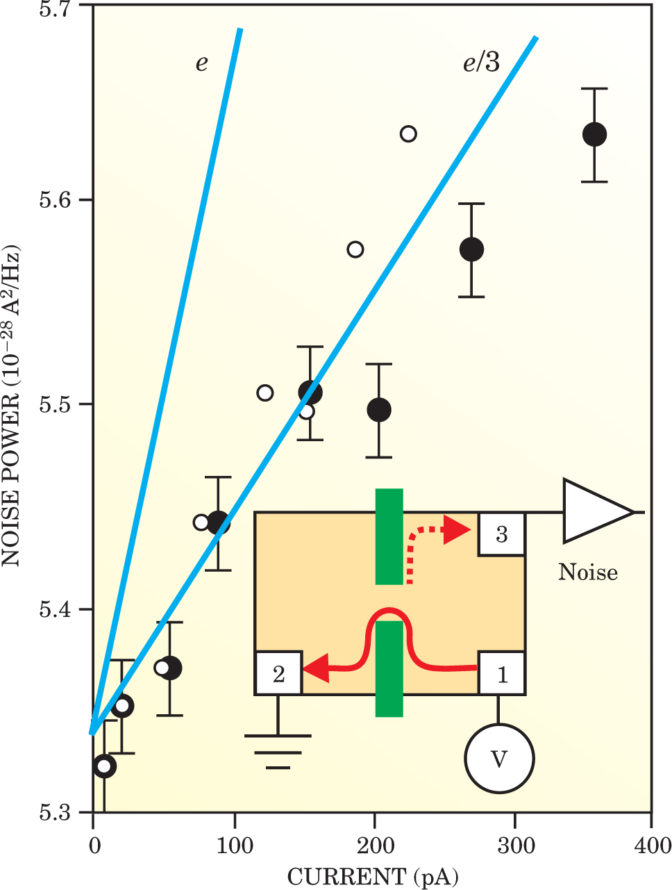
Figure 2. Current noise measured in the fractional quantum Hall regime reveals fractionally charged quasiparticles. The data points with error bars are the measured values at 25 mK and the open circles include a correction for finite tunneling probability. The slopes (in blue) distinguish noise power measured from quasiparticles with charge e/3 and electrons with charge e. The tunneling data fall along the slope corresponding to the fractionally charged quasiparticles. The schematic inset illustrates the experimental setup. Most of the current flows along the lower edge of the 2D electron gas from contact 1 to contact 2 (solid red line), but some quasiparticles tunnel across the split-gate electrode (green) to the upper edge and end up at contact 3 (dashed red line). Researchers first spectrally filtered the current at contact 3, then amplified the signal, and finally measured the mean of the squared fluctuation—the noise power.
(adapted from L. Saminadayar et al., ref. 5)
Quiet electrons
Correlations among electrons reduce the noise below the value
expected for a Poisson distribution of uncorrelated current pulses of charge q = e. Coulomb repulsion is one source of correlations, but in a metal it is strongly screened and ineffective. The dominant source of correlations is the Pauli principle, which prevents double occupancy of an electronic state and leads to Fermi statistics in thermal equilibrium. In a vacuum tube or tunnel junction, the mean occupation of a state is so small that the Pauli principle is inoperative, (and Fermi statistics is indistinguishable from Boltzmann statistics). But that is not the case in a metal.
An efficient way of accounting for the correlations uses Landauer’s description of electrical conduction as a transmission problem. According to the Landauer formula, the time-averaged current
The conductor can be viewed as a parallel circuit of N independent transmission channels with a channel-dependent transmission probability Tn. And one can liken such transmission channels to electromagnetic modes in a waveguide. Tn is formally defined as the nth eigenvalue of the product t · t † of the N × N transmission matrix t and its Hermitian conjugate. In a one-dimensional conductor, which, by definition, has one channel, one would have simply T 1 = |t|2, with t being the transmission amplitude.
The number of channels N is large in a typical metal wire. One has N ≃ A/λ2 F up to a numerical coefficient for a wire with cross-sectional area A and Fermi wavelength λF. Due to the small Fermi wavelength λF ≃ 1 Å of a metal, N is of order 107 for a typical metal wire of width 1 µm and thickness 100 nm. In a semiconductor, typical values of N are smaller but still much larger than 1.
At zero temperature, the noise is related to the transmission probabilities by 6
The factor 1 — Tn describes the reduction of noise due to the Pauli principle. Without it, the noise spectrum would simply reflect the Poisson process, that is, S = S Poisson .
The shot noise formula, shown in equation
The relation S = (2/τ)〈δQ 2〉 between the mean-squared fluctuation of the current and that of the transmitted charge brings us to equation
The quantum shot noise formula shown in equation
A more stringent test used a single-atom junction obtained by the controlled breaking of a thin aluminum wire.
8
The junction is so narrow that the entire current is carried by only three channels (N = 3). The transmission probabilities T 1, T 2, and T 3 could be measured independently from the current-voltage characteristic in the superconducting state of aluminum. By inserting these three numbers (the “pin code” characterizing the junction) into equation
Detecting open transmission channels
The analogy between an electron emitted by a cathode and a bullet shot by a gun works well for a vacuum tube or a point contact, but seems like a rather naive description of the electrical current in a disordered metal or semiconductor. There is no identifiable emission event when current flows through a metal, and one might question the very existence of shot noise. Indeed, for three quarters of a century after the first vacuum tube experiments, not a single measurement existed of shot noise in a metal. A macroscopic conductor (a piece of copper wire, say) shows thermal noise, but no shot noise.
We now understand that, to observe shot noise in a metal, the temperature and length scale requirements are fairly specific: The length L of the wire should be short compared to the inelastic electron-phonon scattering length l in, which becomes longer and longer as one lowers the temperature. For L > l in, each segment of the wire of length l in generates independent voltage fluctuations, with the net result that the shot noise power is reduced by a factor l in/L. Thermal fluctuations, in contrast, are not reduced by inelastic scattering; such scattering only helps establish thermal equilibrium. That explains why, for a long time, only thermal noise could be observed in macroscopic conductors. Incidentally, inelastic electron-electron scattering, which persists to much lower temperatures than electron-phonon scattering, does not suppress shot noise, but rather slightly enhances the noise power. 9
Researchers performing early experiments 10 on mesoscopic semiconducting wires observed the linear relation between noise power and current that is the signature of shot noise, but could not accurately measure the slope. Andrew Steinbach and John Martinis at NIST in Boulder, Colorado, collaborating with Michel Devoret from CEA/Saclay, performed the first quantitative measurement in a thin-film silver wire. 11
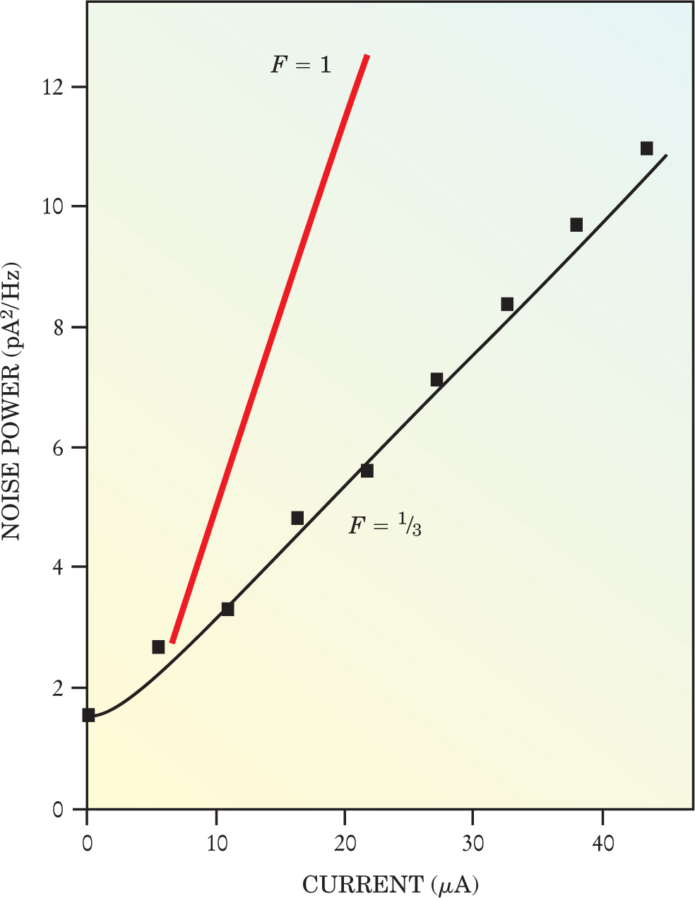
The data shown in figure 3 (from a more recent experiment) presents a puzzle: If we calculate the slope, we find a Fano factor of

Figure 3. Sub-Poissonian shot noise in a disordered gold wire. At low currents, the black curve shows the noise saturate at the level set by the temperature of 0.3 K. Otherwise, the linear relation between noise power and current is the signature of shot noise. The slope is proportional to the Fano factor F, which measures the unit of transferred charge. Poissonian noise would have F = 1, drawn here as the red line. The experimental value F =
(Adapted from M. Henny et al. ref. 11.)
Indeed, electrons in a disordered wire conduct charge diffusively, an entirely different physical process than the tunneling discussed in figure 2. Prior to the experiments, a
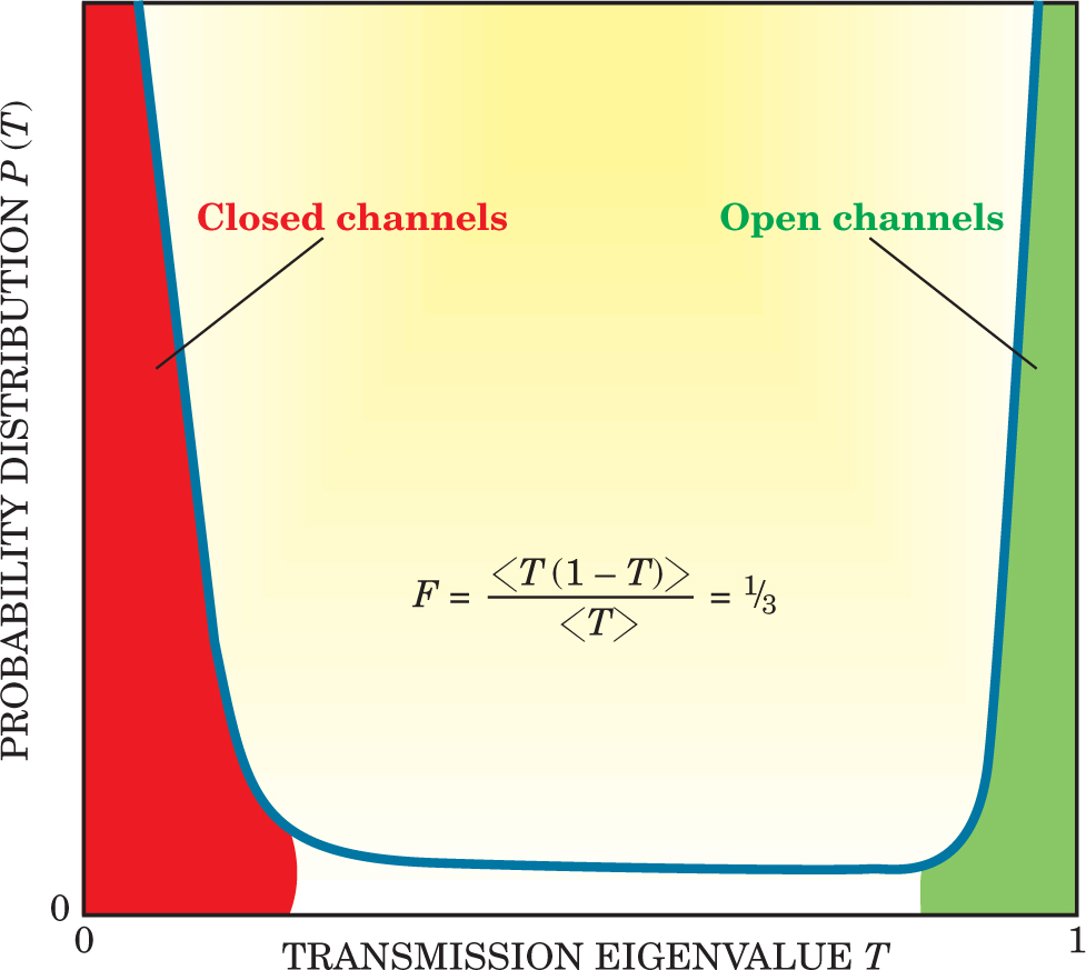
The appearance of open channels in a disordered conductor is surprising. Oleg Dorokhov of the RAS’s Landau Institute for Theoretical Physics in Moscow first noticed the existence of open channels in 1984, but the physical implications were only understood some years later, notably through the work of Yoseph Imry of the Weizmann Institute. The

Figure 4. Bimodal probability distribution of the transmission eigenvalues of a disordered wire, with a peak at 0 for closed channels and a peak at 1 for open channels. The functional form of the distribution (derived by Oleg Dorokhov) is P(T) ∝ T −1(1 — T)−1/2. The
Some experimental demonstrations
3
show the interplay between the doubling of shot noise due to superconductivity and the
Distinguishing particles from waves
So far, we have presented two diagnostic properties of shot noise: It measures the unit of transferred charge in a tunnel junction and it detects open transmission channels in a disordered wire. A third diagnostic property of shot noise is useful in the study of semiconductor microcavities known as quantum dots or electron billiards. These electron billiards are small confined regions in a 2D electron gas, free of disorder, with two narrow openings through which a current is passed. If the shape of the confining potential is sufficiently irregular—and it typically is—the classical dynamics is chaotic and one can search for traces of that chaos in the quantum mechanical properties.
Measuring the shot noise in an electron billiard allows one to distinguish deterministic scattering, characteristic for particles, from stochastic scattering, characteristic for waves. Particle dynamics is deterministic: Initial position and momentum fix the entire trajectory. In particular, they determine whether the particle will be transmitted or reflected, so the scattering is noiseless on all time scales. Wave dynamics is stochastic: The quantum uncertainty in position and momentum introduces a probabilistic element into the dynamics, so it becomes noisy on sufficiently long time scales.
From this qualitative argument, one of us (Beenakker) and van Houten predicted many years ago the suppression of shot noise in a conductor with deterministic scattering. 13 More recently, Oded Agam of the Hebrew University in Jerusalem, Igor Aleiner of SUNY at Stony Brook, and Anatoly Larkin of the University of Minnesota in Minneapolis developed a better understanding, and a quantitative description, of how shot noise measures the transition from particle to wave dynamics. 14 The key concept is the Ehrenfest time, which is the characteristic time scale of quantum chaos.
In classical chaos, the trajectories are highly sensitive to small changes in the initial conditions and are uniquely determined by them. A change δx(0) in the initial coordinate is amplified exponentially in time: δx(t) = δx(0)e αt . Quantum mechanics introduces an uncertainty in δx(0) of the order of the Fermi wavelength λF. One can think of δx(0) as the initial size of a wavepacket. The wavepacket spreads over the entire billiard (of size L) when δx(t) = L. The time at which this happens is called the Ehrenfest time,
The name refers to Paul Ehrenfest’s 1927 principle that quantum mechanical wavepackets follow classical, deterministic, equations of motion. In quantum chaos, that correspondence principle loses its meaning, and the dynamics becomes stochastic on time scales greater than τE. An electron entering the billiard through one of the openings dwells inside, on average, for a time τdwell before exiting again. Whether the dynamics is deterministic or stochastic depends, therefore, on the ratio τdwell/τE. The theoretical expectation for the Fano factor’s dependence on this ratio is plotted in figure 5.

Figure 5. Dependence of the Fano factor F of an electron billiard on the average time τdwell that an electron dwells inside the cavity. The data points were measured in a two-dimensional electron gas confined to an irregularly shaped region, and the solid curve is the theoretical prediction F = 1/4exp(—τE/τdwell) for the transition from stochastic to deterministic scattering, with Ehrenfest time τE = 0.27 ns as a fit parameter. The inset image illustrates the sensitivity to initial conditions of the chaotic dynamics: Tiny variations in the electron’s path (red or green) determine where it exits.
(Adapted from ref. 14 with experimental data from ref. 15.)
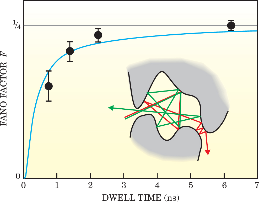
Stefan Oberholzer, Eugene Sukhorukov, and one of us (Schönenberger) 15 conducted an experimental search for the suppression of shot noise by deterministic scattering. An electron billiard (area A ≈ 1 µm2) with two openings of variable width was created in a 2D electron gas by means of gate electrodes. The dwell time, given by τdwell = m*A/ħN, with m* the electron effective mass, was varied by changing the number of modes N transmitted through each of the openings. The experimental data are shown in figure 5.
The Fano factor has the value
Entanglement detector
Sukhorukov, Guido Burkard, and Daniel Loss proposed the fourth and final diagnostic property that we discuss in this overview: shot noise as detector of entanglement. 16
A multiparticle state is entangled if it cannot be factored into a product of single-particle states. Entanglement is the primary resource in quantum computing: Any speed advantage over a classical computer vanishes if the entanglement among electrons is lost, typically through interaction with the environment. (See the articles by John Preskill, Physics Today, June 1999, page 24 , and Barbara Terhal, Michael Wolf, and Andrew Doherty, Physics Today, April 2003, page 46 .) Electron-electron interactions can lead quite naturally to an entangled state, but to use the entanglement in a computation, one would need to spatially separate the electrons without destroying the entanglement. In that respect, the situation in the solid state differs from that in quantum optics, in which the production of entangled photons is a complex operation, whereas their spatial separation is easy.
A pair of quantum dots—each dot containing a single electron—forms the building block for one type of solid-state quantum computer. The strong Coulomb repulsion keeps the electrons separate. The two spins are entangled in the singlet ground state
To appreciate the fundamental difference between “quiet electrons” and “noisy photons,” compare their statistics. Fermi statistics causes the electron noise to be smaller than the Poisson value in equation
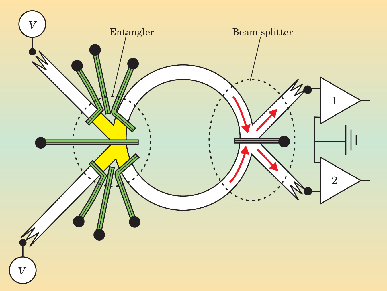
The experiment proposed by the Loss group is sketched in figure 6. The two building blocks are the entangler and the beam splitter. The beam splitter is used to perform the electronic analogue of the optical Hanbury Brown and Twiss experiment. 18 In such an experiment, one measures the cross-correlation of the current fluctuations in the two arms of a beam splitter. Without entanglement, the correlation is positive for photons (bunching) and negative for electrons (antibunching). The observation of a positive correlation for electrons is a signature of the entangled spin-singlet state. In a statistical sense, the entanglement makes the electrons behave like photons.

Figure 6. Production and detection of a spin-entangled electron pair. The double quantum dot (yellow) is defined by gate electrodes (green) on a two-dimensional electron gas. The two voltage sources at the far left inject one electron into each dot, which results in an entangled spin-singlet ground state. A voltage pulse on the gates then forces the two electrons to enter opposite arms of the ring. Scattering (red arrows) of the electron pair by a tunnel barrier creates shot noise, measured by amplifiers (1,2) in each of the two outgoing leads at the far right. The observation of a positive correlation between the current fluctuations at each amplifier is a signature of the entangled spin-singlet state.
(Figure courtesy of L. P. Kouwenhoven and A. F. Morpurgo, Delft University of Technology.)
An alternative to the proposal shown in figure 6 is to start with Cooper pairs in a superconductor, which are also in a spin-singlet state. 16 The Cooper pairs can be extracted from the superconductor and injected into a normal metal by applying a voltage across a tunnel barrier at the metal-superconductor interface.
The experimental realization of one of those two theoretical proposals would open up a new chapter in the use of noise to probe quantum mechanical properties of electrons. Although that range of applications is still in its infancy, the field as a whole has progressed far enough to prove Landauer right: There is a signal in the noise.
References
1. For an overview of the literature on quantum shot noise, see Ya. M. Blanter, M. Büttiker, Phys. Rep. 336, 1 (2000) https://doi.org/10.1016/S0370-1573(99)00123-4 .
2. F. Lefloch, C. Hoffmann, M. Sanquer, D. Quirion, Phys. Rev. Lett. 90, 067002 (2003) https://doi.org/10.1103/PhysRevLett.90.067002 .
3. A. A. Kozhevnikov, R. J. Schoelkopf, D. E. Prober, Phys. Rev. Lett. 84, 3398 (2000) https://doi.org/10.1103/PhysRevLett.84.3398
X. Jehl, M. Sanquer, R. Calemczuk, D. Mailly, Nature 405, 50 (2000) https://doi.org/10.1038/35011012 .4. C. L. Kane, M. P. A. Fisher, Phys. Rev. Lett. 72, 724 (1994) https://doi.org/10.1103/PhysRevLett.72.724 .
5. L. Saminadayar, D. C. Glattli, Y. Jin, B. Etienne, Phys. Rev. Lett. 79, 2526 (1997) https://doi.org/10.1103/PhysRevLett.79.2526
R. de-Picciotto, M. Reznikov, M. Heiblum, V. Umansky, G. Bunin, D. Mahalu, Nature 389, 162 (1997) https://doi.org/10.1038/38241
M. Reznikov, R. de-Picciotto, T. G. Griffiths, M. Heiblum, V. Umansky, Nature 399, 238 (1999) https://doi.org/10.1038/20384 .6. V. A. Khlus, Sov. Phys. JETP 66, 1243 (1987)
G. B. Lesovik, JETP Lett. 49, 592 (1989)
M. Büttiker, Phys. Rev. Lett. 65, 2901 (1990) https://doi.org/10.1103/PhysRevLett.65.2901 .7. L. S. Levitov, G. B. Lesovik, JETP Lett. 58, 230 (1993).
8. R. Cron, M. F. Goffman, D. Esteve, C. Urbina, Phys. Rev. Lett. 86, 4104 (2001) https://doi.org/10.1103/PhysRevLett.86.4104 .
9. K. E. Nagaev, Phys. Rev. B 52, 4740 (1995) https://doi.org/10.1103/PhysRevB.52.4740
V. I. Kozub, A. M. Rudin, Phys. Rev. B 52, 7853 (1995) https://doi.org/10.1103/PhysRevB.52.7853 .10. F. Liefrink, J. I. Dijkhuis, M. J. M. de Jong, L. W. Molenkamp, H. van Houten, Phys. Rev. B 49, 14066 (1994) https://doi.org/10.1103/PhysRevB.49.14066 .
11. A. H. Steinbach, J. M. Martinis, M. H. Devoret, Phys. Rev. Lett. 76, 3806 (1996) https://doi.org/10.1103/PhysRevLett.76.3806 .
More recent experiments include R. J. Schöelkopf, P. J. Burke, A. A. Kozhevnikov, D. E. Prober, M. J. Rooks, Phys. Rev. Lett. 78, 3370 (1997) https://doi.org/10.1103/PhysRevLett.78.3370
M. Henny, S. Oberholzer, C. Strunk, C. Schönenberger, Phys. Rev. B 59, 2871 (1999) https://doi.org/10.1103/PhysRevB.59.2871 .12. C. W. J. Beenakker, M. Büttiker, Phys. Rev. B 46, 1889 (1992) https://doi.org/10.1103/PhysRevB.46.1889
K. E. Nagaev, Phys. Lett. A 169, 103 (1992) https://doi.org/10.1016/0375-9601(92)90814-3 .13. C. W. J. Beenakker, H. van Houten, Phys. Rev. B 43, 12066 (1991) https://doi.org/10.1103/PhysRevB.43.12066 .
14. O. Agam, I. Aleiner, A. Larkin, Phys. Rev. Lett. 85, 3153 (2000) https://doi.org/10.1103/PhysRevLett.85.3153 .
15. S. Oberholzer, E. V. Sukhorukov, C. Schönenberger, Nature 415, 765 (2002) https://doi.org/10.1038/415765a .
16. G. Burkard, D. Loss, E. V. Sukhorukov, Phys. Rev. B 61, 16303 (2000) https://doi.org/10.1103/PhysRevB.61.R16303 .
The alternative entangler using Cooper pairs is described in M.-S. Choi, C. Bruder, D. Loss, Phys. Rev. B 62, 13569 (2000) https://doi.org/10.1103/PhysRevB.62.13569
G. B. Lesovik, T. Martin, G. Blatter, Eur. Phys. J. B 24, 287 (2001) https://doi.org/10.1007/s10051-001-8675-4 .17. A. W. Holleitner, R. H. Blick, A. K. Hüttel, K. Eberl, J. P. Kotthaus, Science 297, 70 (2002) https://doi.org/10.1126/science.1071215
W. G. van der Wiel, S. De Franceschi, J. M. Elzerman, T. Fujisawa, S. Tarucha, L. P. Kouwenhoven, Rev. Mod. Phys. 75, 1 (2003) https://doi.org/10.1103/RevModPhys.75.1 .18. M. Henny, S. Oberholzer, C. Strunk, T. Heinzel, K. Ensslin, M. Holland, C. Schönenberger, Science 284, 296 (1999) https://doi.org/10.1126/science.284.5412.296
W. D. Oliver, J. Kim, R. C. Liu, Y. Yamamoto, Science 284, 299 (1999) https://doi.org/10.1126/science.284.5412.299 .
More about the authors
Carlo Beenakker is a professor of theoretical physics at the Lorentz Institute of Leiden University in the Netherlands. Christian Schönenberger is a professor of physics at the University of Basel in Switzerland.
Carlo Beenakker, 1 Lorentz Institute of Leiden University, Netherlands .
Christian Schönenberger, 2 University of Basel, Switzerland .


