Minimalist model captures water-cycle complexities
DOI: 10.1063/PT.3.1242
Images taken 18 August 2009 from a European Space Agency satellite stationed in a geosynchronous orbit above the equator and prime meridian show a typical pattern of cloud cover off Africa’s west coast. Sprawling marine stratocumulus clouds are visible in two familiar forms: a so-called closed-cellular field, a densely packed layer of clouds separated by thin rings of clear sky; and a more sparsely populated open-cellular field, a honeycomb-like lattice of rings of clouds encircling large pockets of clear sky.
When scientists led by Graham Feingold (National Oceanic and Atmospheric Administration, Boulder, Colorado) zoomed in on the satellite images, they saw intriguing behavior. 1 After accounting for wind advection, they noticed that now and then, a cloud in the open-cellular field would vanish, leaving clear sky. Kilometers away, a new cloud would form. Every hour or so, the disappearing act would repeat.
The oscillations Feingold and his colleagues observed are among several surprising dynamical phenomena seen in the water cycle. Meteorologists have also witnessed abrupt changes in cloud morphology and seemingly unprovoked transitions from drizzles to downpours. Although such complexities affect long-term climate trends—they play a part in determining Earth’s albedo as well as the distribution and intensity of rainfall events—most climate models gloss over them in the name of computational efficiency.
More sophisticated models such as large-eddy simulation (LES) strive to incorporate as much physical detail as possible by coupling cloud microphysics with fluid dynamics. Aided by LES, Feingold and company were able to replicate the oscillations they had seen in the satellite images; their explanation—that rainfall reverses the convection patterns—is detailed in figure 1.

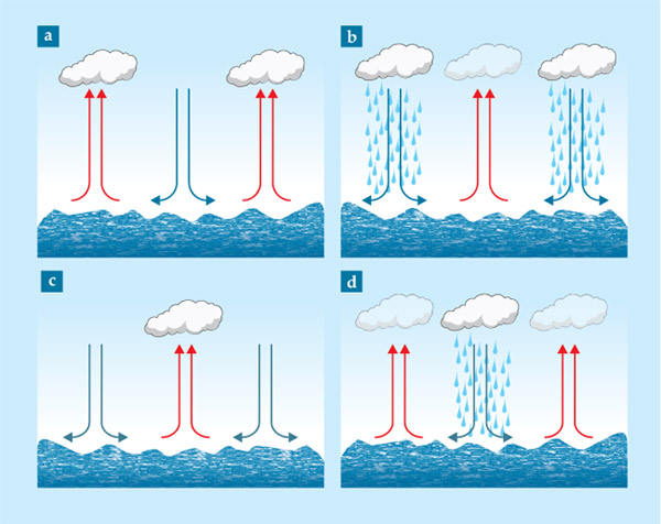
Figure 1. Some marine stratocumulus clouds seem to periodically vanish and reappear, possibly via the mechanism illustrated here. (a) Thermal convection circulates warm air (red arrows) upward and cool air (blue arrows) downward, with the updrafts producing clouds. (b) As the clouds precipitate, evaporative cooling reverses the convective pattern, creating a new updraft, and a new cloud, several kilometers away. (c) With the original clouds converted entirely to rain, a new cloud hovers above the new updraft of warm air. (d) As rain falls from the newly formed cloud, the patterns again reverse, and the cycle repeats.
But the extensive detail of an LES can mask underlying patterns. It doesn’t explain, for example, why some cloud-precipitation systems seem to oscillate and others remain steady. Now, inspired by a 100-year-old model of a predator–prey ecosystem, Feingold and coauthor Ilan Koren (Weizmann Institute of Science, Rehovot, Israel) have captured some of the water cycle’s complexity—including behavior related to the oscillating clouds—in a model simple enough for pen-and-paper analysis. 2
The water cycle
Koren and Feingold are mainly interested in liquid water clouds, formed when water vapor—supplied mostly by evaporation at Earth’s surface and carried upward by thermal convection—creates supersaturated conditions in cooler regions of the atmosphere. There, the water vapor condenses into the liquid droplets that make up a cloud, with aerosol particles serving as the condensation nuclei. Once cloud droplets have grown to about 40 microns in diameter, condensation gives way to coalescence, and the droplets begin the 10- to 20-minute-long process of aggregating into a raindrop heavy enough to fall out of the sky.
To translate that conceptual picture of the water cycle into a viable quantitative prediction, one needs to account for a host of environmental factors—surface and atmospheric temperature fluctuations, aerosol concentration, and prevailing winds, to name a few. LES is up to that task, but to simulate rainfall in a column of troposphere just 12 km × 12 km across, an LES would require solving a system of order 107 equations. “To model clouds from the bottom up, you have to address length scales spanning more than 12 orders of magnitude,” says Koren.
Koren and Feingold sacrificed much of that detail, seeking instead to ferret out emergent structures—the system-wide patterns that develop as a result of local interactions. Their philosophy, Koren recalls, was “to zoom out, not in.”
Predators and prey
Koren and Feingold drew inspiration from the nearly century-old Lotka–Volterra model of a two-species, predator–prey ecosystem. Lotka and Volterra’s assumptions were succinct: (1) Prey reproduce, and predators die off, at rates proportional to their respective populations. (2) Predators consume prey at a rate proportional to the product of their respective populations.
The simple mathematical expressions that result yield surprisingly rich dynamical outcomes. For instance, it’s possible for predator and prey to coexist in a steady state, with predators eating just enough prey to maintain their own number, and prey reproducing at just the rate needed to maintain theirs.
But it’s also possible that predators could set out greedily, devouring their prey to near extinction. With their sole food source diminished, the predators’ population plummets as well. For a time, that frees the few remaining prey to reproduce with minimal hindrance, until they once again constitute an ample food supply. Then the predators flourish anew, and the cycle repeats.
That perpetual back-and-forth is one form of what’s known as a limit cycle. Plotted against time, the two species’ populations oscillate indefinitely, with the predator population lagging a quarter cycle behind that of the prey.
Koren and Feingold’s LES results suggested that precipitation systems might exhibit similar limit cycles. Adopting the Lotka–Volterra equations as a template, they set out to construct a dynamical model that would accommodate not predators and prey, but clouds, precipitation, and aerosol particles.
Minimalist mathematics
The researchers noted that clouds, like Lotka and Volterra’s prey, tend to form and grow gradually with time—mainly due to the natural upward convection of warm moist air. And like predators, precipitation eats away at the cloud layer yet relies on that same layer to sustain itself. Aerosol particles mediate the precipitation–cloud interactions: The higher the aerosol concentration, the more numerous the water droplets and the longer it takes for the droplets to grow large enough to coalesce into rain. To put it in predator–prey vernacular, the hunt becomes more challenging.
Building on those basic concepts, the researchers distilled the cloud-aerosol-precipitation system into a system of three equations. Although the equations differ from Lotka and Volterra’s predator–prey model, the solutions exhibit similarly rich dynamics.
The model predicts that aerosol-rich skies should eventually settle into a steady state like that shown in figure 2a, with a light drizzle of rain offsetting the formation of new cloud droplets. Aerosol-deficient clouds, on the other hand, are likely to precipitate faster than they can replenish themselves and collapse into a downpour of rain.

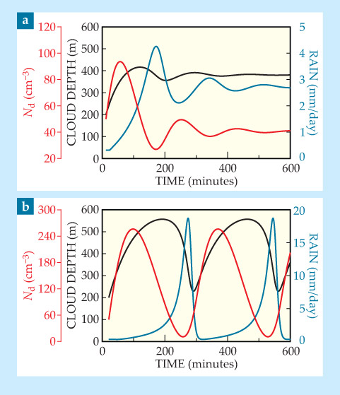
Figure 2. Steady states and limit cycles. (a) The time evolution of a model water cycle shows cloud-layer thickness (black), aerosol concentration Nd (red), and rain rate (blue) settling to a steady state. (b) Modeled under slightly different conditions—with different characteristic time scales for cloud buildup, aerosol-particle buildup, and droplet coalescence—the system enters a repeating cycle, with gradual buildups of cloud thickness and aerosol concentration punctuated by brief bouts of strong rain. (Adapted from ref.
The team’s model also suggests the possibility of limit cycles like the one shown in figure 2b, with periods of gradual cloud growth punctuated by brief bouts of heavy rain. But whereas the steady state and unstable collapse have been documented in field observations, evidence in support of limit cycles—outside of LES results and anecdotal data—remains scarce. “We hope to strengthen that aspect of the study with observations,” says Feingold, “but the measurements aren’t easy.”
Still, Feingold sees the pared-down model as a potentially valuable complement to LES-type approaches: “We don’t want to discard all of the details. But to the extent that we can, we think it’s also worth trying to use simple models to see the bigger picture.”
References
1. G. Feingold et al., Nature 466, 849 (2010). https://doi.org/10.1038/nature09314
2. I. Koren, G. Feingold, Proc. Natl. Acad. Sci. USA 108, 12227 (2011). https://doi.org/10.1073/pnas.1101777108


