Helioseismology plumbs new depths

For more than two decades, solar astronomers have known that the magnetized plasma at the Sun’s surface gradually drifts from the equator to the poles. It follows, then, that somewhere in the solar interior that plasma must return to the equator—after all, the Sun’s poles do not become more massive with time. But whereas surface velocities can be detected by line-of-sight Doppler shifts, advection of passive tracers, and other straightforward means, interior flows are hidden by the Sun’s opaque photosphere. As a result, the meridional return flow has long eluded definitive detection.

Hints of an equatorward flow can be seen in the motion of so-called supergranules, convection cells that cycle plasma between the Sun’s interior and its surface. The smallest supergranules drift poleward, presumably carried by surface currents. But some larger granules can be seen to move upstream, toward the equator. One theory is that the larger cells penetrate deeper into the solar interior and therefore may be getting caught in the equatorward undertow. Based on that theory and a few simplifying assumptions, David Hathaway of NASA’s Marshall Space Flight Center in Huntsville, Alabama, estimated last year ¹ that the meridional flow turns equatorward at a depth of about 50 Mm, about 1/14 the solar radius R_⊙.

Junwei Zhao of Stanford University in Palo Alto, California, and coworkers there and at NASA’s Goddard Space Flight Center in Greenbelt, Maryland, have now detected the equatorward return using a more direct and precise technique: time–distance helioseismology. ² Analogous to terrestrial seismology, helioseismology uses correlations between surface acoustic waves to infer properties of the solar interior. (See the article by John Harvey, Physics Today, October 1995, page 32 .) The technique has been around for decades, but recent refinements and improved observational data have allowed Zhao and coworkers to probe meridional velocities to depths of 170 Mm, nearly ¼ the way to the Sun’s center. And in a result that’s bound to baffle some solar-dynamo theorists, the researchers find not one flow reversal but two.

Solar echoes

Virtually all solar plasma flow occurs in an outer shell known as the convective zone, which spans radial distances between 0.7 R_⊙ and the solar surface. The complex, three-dimensional flows in the convective zone help transport heat generated in the solar core to the cool surface and give rise to the dynamo that’s responsible for the Sun’s magnetic dipole and 11-year activity cycle. (For more on magnetic dynamos, see the article by Daniel Lathrop and Cary Forest, Physics Today, July 2011, page 40 , and the article by Peter Olson on page 30 in this issue.) Beneath the convective zone, the Sun is essentially a uniformly spinning ball of gas.

Meridional flows in the convective zone are difficult to detect in part because they’re relatively small. Whereas mean rotation speeds and velocity fluctuations are typically around 1 km/s, the net meridional flow peaks at around 10–20 m/s. In the 1990s Thomas Duvall Jr, a solar astronomer at NASA Goddard, and coworkers introduced time-distance helioseismology as one way to detect the subtle flows. ³

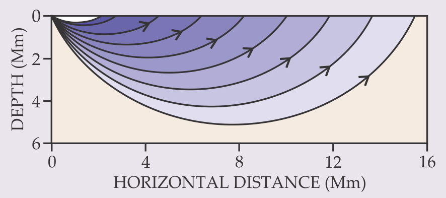
Like all helioseismology techniques, time–distance helioseismology takes advantage of the fact that local density and temperature—and, therefore, the speed of sound—increase with depth in the solar interior. As a result, acoustic waves that propagate into the solar interior refract and bend back toward the surface. Treated as rays, they trace arcs like those depicted in figure 1. On reaching the surface, the rays are then reflected back into the interior; the depth of the trajectory is roughly proportional to the distance Δ between surface reflections.

Duvall’s strategy was to cross correlate acoustic signals at points along a meridian to determine time lags between surface reflections as a function of Δ. Acoustic rays travel faster with subsurface currents than against them, so meridional flow velocities along a ray trajectory can be inferred from slight differences between north–south and south–north lag times. The effect is subtle: For deep trajectories, the flow may shave or add less than one second per hour of travel time. Nonetheless, with enough data and an appropriate model of the solar interior, one can rather precisely infer subsurface velocity profiles.

Starting in the 1990s, the Stanford group began applying Duvall’s time–distance helioseismology approach to acoustical data collected by the Michelson Doppler Imager, which was launched aboard the Solar and Heliospheric Observatory in 1995. Those studies clearly showed the poleward velocity growing smaller with depth, but they failed to find a reversal.

Center-to-limb effect

Last year, Zhao and his coworkers began analyzing data from the recently launched Solar Dynamics Observatory’s Helioseismic and Magnetic Imager (HMI) with the hope that the instrument’s higher-resolution images might allow deeper and more accurate measurements of the meridional profile. Soon, however, they encountered a troubling inconsistency.

Surface oscillations can be detected in solar images via a number of observables; they show up as changes in surface brightness or as oscillations in the Doppler shifts of various spectral lines, for instance. In principle, all those observables should carry identical acoustic information. But the Stanford researchers were finding different results for each observable. “For months, we thought that our approach might have been fundamentally flawed,” recalls Zhao. “It was very discouraging.”

As a check, the team calculated eastward velocities along the Sun’s equator using HMI images collected over a 10-day span in December 2010. ⁴ Those velocities should be independent of longitude, but the group’s analysis indicated larger-than-average velocities in the right, or eastern, half of the solar disk and smaller-than-average velocities in the left. Something was creating the illusion of an extra velocity component—in some cases as large as 10 m/s—directed from the center of the solar disk to its limb.

Zhao and his colleagues concluded that the discrepancy had to have been a systematic error. Assuming it affects meridional measurements in the same way it does equatorial ones, it would artificially bias flow velocities toward the poles and potentially mask any equatorward flow. Indeed, when the researchers subtracted the center-to-limb components from meridional profiles calculated with different observables, the resulting profiles were all consistent with one another. “We still don’t understand what’s causing the effect,” says Zhao. “But the correction method appears to be robust.”

The Sun’s conveyor belts

In the new work, the researchers applied the center-to-limb correction to a helioseismology analysis of two years of HMI data. Figure 2a shows resulting flow profiles averaged over 10°-wide latitudinal bands in the Sun’s northern and southern hemispheres. Two distinct reversals can be seen, at radial distances of about 0.9 R_⊙ and 0.8 R_⊙. Such profiles imply a large-scale flow field consisting of two distinct circulation cells, as illustrated in figure 2b.

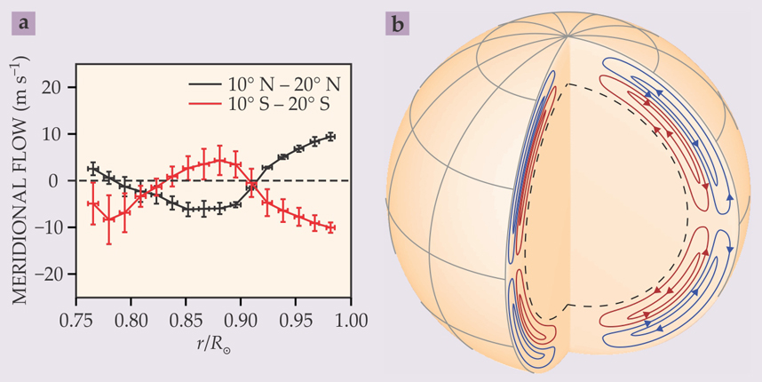
A two-cell meridional circulation doesn’t come as a complete surprise. Other researchers have speculated on its existence from indirect experimental evidence and numerical simulations. “But this new evidence is currently the most compelling,” says Mark Miesch of the National Center for Atmospheric Research in Boulder, Colorado.

The results could prove problematic for some solar dynamo theories. In particular, one popular class of models—the so-called flux-transport dynamo models—has long relied on a single circulation cell to explain phenomena associated with the 11-year solar activity cycle. ⁵ For instance, sunspots—cool, dark patches on the solar surface that form when magnetized plasma bubbles up from the convective zone’s floor—appear at mid latitudes early in the cycle and at progressively lower latitudes as the cycle proceeds.

Flux-transport dynamo models attribute that equatorward migration to the meridional flow at the bottom of the convective zone. But in a two-cell pattern—or any even-celled pattern—that flow is toward the poles, not the equator.

A potential saving grace for the flux-transport models is the possibility of a third meridional cell squeezed in between 0.7 R_⊙, the radial distance of the convective-zone floor, and 0.75 R_⊙, the distance corresponding to Zhao and coworkers’ deepest measurements. The HMI will continue collecting data for at least three more years, which should allow Zhao and his coworkers to extend their measurements deeper, perhaps to the convective zone’s floor. If those studies don’t reveal a third reversal, there may be little wiggle room left for flux-transport dynamo models of the solar cycle.

References

1. D. H. Hathaway, Astrophys. J. 760, 84 (2012). https://doi.org/10.1088/0004-637X/760/1/84
2. J. Zhao, et al., Astrophys J. Lett. 774, L29 (2013).https://doi.org/10.1088/2041-8205/774/2/L29
3. T. L. Duvall et al., Nature 362, 430 (1993). https://doi.org/10.1038/362430a0
4. J. Zhao et al., Astrophys. J. Lett. 749, L5 (2012). https://doi.org/10.1088/2041-8205/749/1/L5
5. M. Dikpati, P. Charbonneau, Astrophys. J. 518, 508 (1999).https://doi.org/10.1086/307269