Circulation collapses in turbulent liquid metals

Earth’s magnetic field—useful not just for navigation but for shielding the planet’s surface from the charged particles of the solar wind—owes its existence to the convective flow of the outer core. Heated from below and cooled from above, the churning liquid iron–nickel alloy hosts a self-sustaining dynamo in which electric currents and magnetic fields continually induce one another.

But the full picture is not so simple. The flow in Earth’s core is almost certainly turbulent—and therefore chaotic, nonlinear, and hard to model. Observing the flow directly is impossible. And modelers get their simulations to output an Earth-like field only when they input material parameters, such as viscosity, that they know are wrong. (See the article by Daniel Lathrop and Cary Forest, Physics Today, July 2011, page 40 .) Clearly, something is missing from researchers’ understanding of liquid-metal turbulence.

Now Tobias Vogt, of the Helmholtz-Zentrum Dresden-Rossendorf (HZDR) in Germany, and colleagues have identified what may be an important piece of the puzzle. In a 64-cm-tall cylinder, shown in figure 1, they studied turbulent convection of a gallium-indium-tin (GaInSn) mixture that’s liquid at room temperature.

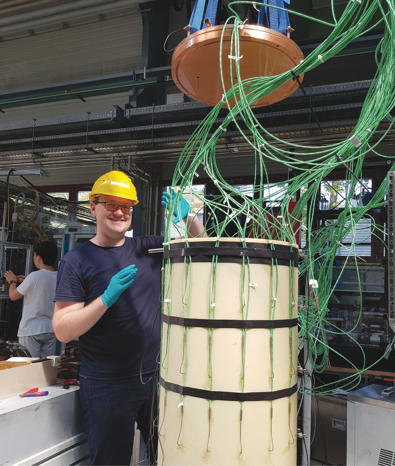
Figure 1.

What they found was completely unexpected. Instead of a stable large-scale circulation—one or a few big swirling vortices that fill the entire container and persist over time—they saw a constantly changing flow structure dominated by smaller, fleeting features. ¹

Until now, large-scale circulation has been considered an inevitable and ubiquitous feature of turbulent convection. Its absence in the HZDR liquid-metal experiments was not predicted by any theory. It’s too soon to say exactly what Vogt and colleagues’ observation means for understanding Earth’s core and other planetary dynamos. But there could be profound implications for how turbulent liquid metals transport heat and momentum, especially at large length scales.

Listen in

There are good reasons to think that turbulence in liquid metals is fundamentally different from turbulence in other fluids. Convective turbulence involves the interplay between the fluid’s velocity field and its temperature field, so it’s governed by the relative sizes of the features—vortices and thermal hot spots—that the fluid can sustain over time. For many fluids, the features are about the same size, but for liquid metals, the high thermal conductivity quickly washes out any small-scale temperature gradients. The difference is quantified by a dimensionless material property called the Prandtl number: on the order of 1–10 for typical liquids and gases, but just 0.03 for GaInSn.

Liquid metals are difficult to study in the lab. They’re expensive, heavy, and hard to work with. They’re also opaque, so the light-based methods used to study turbulence in other fluids (see, for ex

ample, the article by Leo Kadanoff, Physics Today, August 2001, page 34 ) are inapplicable.

But all is not lost. For decades the HZDR magnetohydrodynamics department has been working to develop, refine, and apply techniques for measuring velocity fields in liquid metals. In addition to turbulent convection and planetary cores, HZDR researchers are also interested in industrial applications—optimizing metallurgical processes and even exploring possibilities for liquid-metal batteries.

Light doesn’t penetrate liquid metals, but sound does, so one of the HZDR team’s go-to methods is ultrasound Doppler velocimetry (UDV): using ultrasound transducers to measure the velocity profiles of tiny acoustically reflective oxide particles that permeate the liquid metal. Technical limitations make it hard to deploy more than about 20 transducers simultaneously, and each one measures the profile only along a one-dimensional cut through the system, as shown in figure 2a. But the direct velocity measurements, especially when tracked over time, give the researchers some idea of the flow structure.

Figure 2.

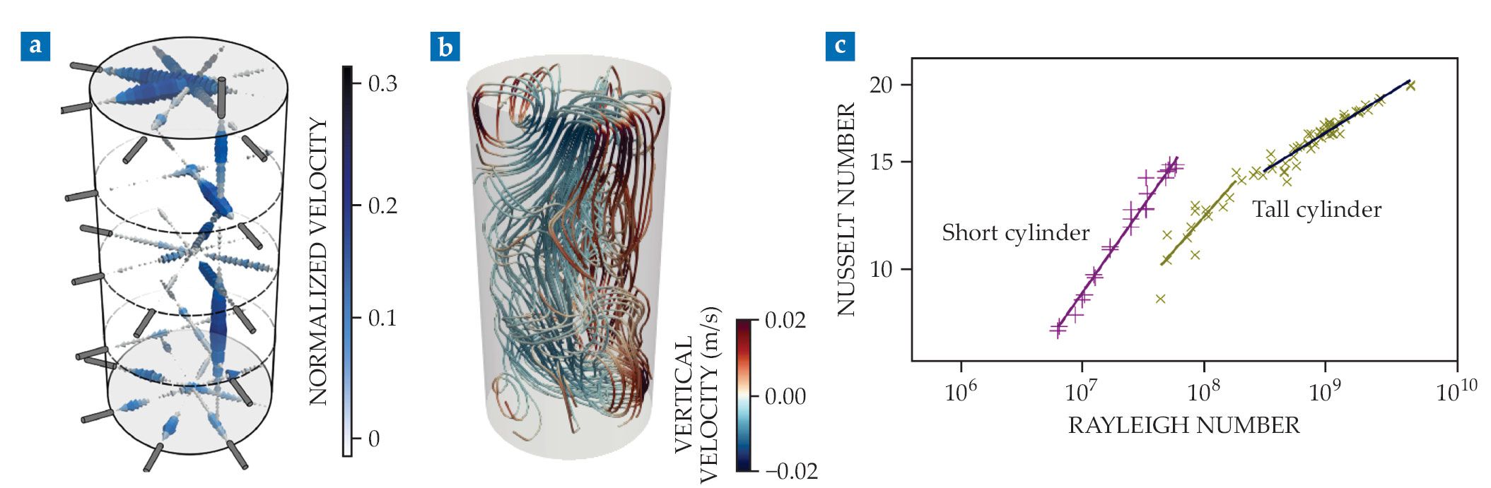
For a more complete picture, the HZDR team developed a complementary technique called contactless inductive flow tomography (CIFT). In a CIFT measurement, flowing metal is placed in a weak magnetic field—not strong enough to disrupt the flow but strong enough to induce eddy currents. ² The currents generate their own magnetic field, which is measured with magnetometers surrounding the sample. By solving a sophisticated inverse problem, the researchers can convert their magnetic measurements into a reconstruction of the 3D flow.

Although CIFT potentially offers much more detailed insight into a flow structure, it’s also a lot more work. So the researchers typically start their studies with UDV measurements and turn to CIFT only when they know it will be worth the effort. Vogt and colleagues’ published analysis is based on their UDV studies. But in the time since they submitted their paper last year, they’ve begun some preliminary CIFT measurements, including the one shown in figure 2b. Both experimental techniques show the collapse of the large-scale circulation, with the liquid-metal flow devolving into smaller, fast-changing, incoherent structures.

Great heights

To classify different regimes of turbulent convective flow, another important dimensionless number is the Rayleigh number. Unlike the Prandtl number, which is an inherent property of the fluid, the Rayleigh number also depends on the experimental conditions and geometry: It’s proportional to the container height to the fourth power times the overall temperature gradient. (Equivalently, it’s proportional to the temperature difference across the system times the height cubed.) The temperature gradient is what drives the convection; to become turbulent, the flow needs to overcome resistance imposed by the fluid’s viscosity and thermal conductivity, each of which introduces a factor of the height squared.

Earth’s outer core is more than 2000 km thick, so its Rayleigh number is many orders of magnitude larger than can possibly be studied in a lab or simulated on any present-day computer. In their push to higher Rayleigh numbers, Vogt and colleagues chose to use a cylinder taller than it is wide, so they could make the best use of their costly and cumbersome GaInSn. In their previous work on convective turbulence, they’d always used containers as wide or wider than they are tall. All those systems—by necessity, much shorter than 64 cm—featured stable, large-scale circulation. ³

To estimate how turbulence might behave in systems too large for a lab experiment, researchers look for trends as a function of the Rayleigh number. For a single experimental setup, they can obtain a range of Rayleigh numbers by varying the temperature difference across the fluid. Because liquid metals transport heat so easily, it’s difficult for them to sustain large temperature gradients. But with the help of powerful heaters and coolers, Vogt and colleagues realized temperature differences from 0.25 K to 51.2 K across their tall cylinder, for Rayleigh numbers of 2 × 10⁷ up to 5 × 10⁹.

The key thermodynamic output is the Nusselt number, roughly the ratio of the amount of heat transported by convection to the amount that would have been transported by conduction alone if the fluid were at rest. For turbulent flows, the Nusselt number is greater than 1, even in liquid metals—despite the high thermal conductivity, the majority of heat is transported by convection. And as the Rayleigh number increases, so does the Nusselt number. The question is, how quickly?

For a given fluid and experimental geometry, the Nusselt number is usually a power-law function of the Rayleigh number with an exponent somewhere between about 0.2 and 0.5, depending on the system. If the scaling isn’t well characterized by a single exponent, then it can often be described by a sum of terms with different exponents, with the effect that the dominant exponent increases with increasing Rayleigh number. ⁴

But that’s not what Vogt and colleagues observed. Rather, as seen in the green data in the log–log plot in figure 2c, they found a lower power-law exponent for higher Rayleigh numbers. For Rayleigh numbers below 2 × 10⁸, the exponent was 0.22: on the low side, but within the expected range. But for higher Rayleigh numbers, the exponent dropped to 0.124—a lower value than had been predicted by any theory or observed before in any other experiment.

Scaling up

If the low-exponent power law could be extended indefinitely to higher Rayleigh numbers, it would suggest that Earth’s core convection transfers far less heat than previously expected—and that it probably differs from expectations in other ways too. But far too many dots remain unconnected to confidently make such a simple extrapolation.

The HZDR researchers don’t yet have a clear understanding of exactly what’s going on at the Rayleigh numbers they observed, let alone at the ones they didn’t. They tentatively attribute the change in power-law exponent at the Rayleigh number of 2 × 10⁸ to a transition from a partially decoherent regime of turbulent flow to a fully decoherent one. But their observations of the turbulent flows are still too spotty to draw any solid conclusions.

Experimenters often turn to computer simulations to fill in the gaps in their measurements, but Vogt and colleagues don’t have that option. A huge amount of computing power is necessary to simulate all the tiny vortices of high-Rayleigh-number, low-Prandtl-number flows. Meaningful results are possible only up to Rayleigh numbers of about 10⁹. Vogt and colleagues’ experiments are already past that threshold.

But with the confirmation that liquid metals’ strange behavior is within experimental reach, the HZDR researchers are pressing on with their measurements. To push further into the unexplored regimes of turbulent liquid metals, they’re in the process of setting up a new lab to perform experiments on liquid sodium. Despite that material’s hazards, it’s available in larger quantities—the researchers have 12 cubic meters of it ready to go—and has a Prandtl number an order of magnitude lower than GaInSn’s.

References

1. F. Schindler et al., Phys. Rev. Lett. 128, 164501 (2022). https://doi.org/10.1103/PhysRevLett.128.164501
2. F. Stefani et al., IOP Conf. Ser.: Mat. Sci. Eng. 143, 012023 (2016). https://doi.org/10.1088/1757-899X/143/1/012023
3. See, for example, T. Vogt et al., Proc. Natl. Acad. Sci. USA 115, 12674 (2018). https://doi.org/10.1073/pnas.1812260115
4. S. Grossmann, D. Lohse, J. Fluid Mech. 407, 27 (2000). https://doi.org/10.1017/S0022112099007545
More about the authors
Johanna L. Miller, jmiller@aip.org