Zero-field nuclear magnetic resonance
DOI: 10.1063/PT.3.1948
Progress in nuclear magnetic resonance (NMR) spectroscopy and magnetic resonance imaging (MRI) is conventionally associated with working at higher and higher magnetic fields. Although such fields certainly have their virtues, those virtues come with a price, literally and figuratively. A typical high-field setup costs on the order of $1 million, requires constant cryogenic maintenance, is immobile, and can’t be used on samples with metallic inclusions or implanted devices. MRI, for example, has long been off-limits to patients with pacemakers, which can malfunction under strong magnetic fields. Also, larger magnets often require extensive magnetic field shimming to produce the spatially uniform fields needed to obtain high-resolution spectra.
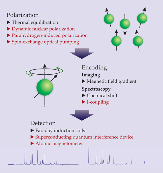
Starting with the pioneering work of Alexander Pines and coworkers in the 1980s, 1 however, a somewhat unexpected trend has developed toward using ultralow, submicrotesla fields—or even no external field at all. That trend has been enabled by new techniques and technologies that have relaxed the requirement for large magnetic fields in each of the three main stages of an NMR experiment—polarization, encoding, and detection (see figure 1).

Figure 1. The three stages of a nuclear magnetic resonance experiment, with representative techniques. In the traditional approach, a sample’s nuclear spins are polarized via thermal equilibration in a strong magnetic field; information about molecular structure or spatial distribution of nuclei is encoded in the form of spin resonances—for instance, by way of chemical shifts or an applied magnetic field gradient; and the resonances are detected with Faraday induction coils. Each stage benefits from a strong magnetic field. In the absence of such a field (techniques in red), spin polarization can be achieved by dynamic nuclear polarization, spin-exchange optical pumping, or parahydrogen-induced polarization; encoding can take the form of J-coupling; and spin resonances can be detected using superconducting quantum interference devices or atomic magnetometers.
In traditional, high-field NMR, a sample’s nuclear spins are polarized via thermal equilibration in a magnetic field. The degree of spin polarization is proportional to the magnitude of the field, inversely proportional to temperature, and usually small. Spin-1⁄2 hydrogen nuclei (protons) at room temperature in a 1-T magnetic field—typical conditions for an MRI experiment—attain polarizations on the order of 10 parts per million.
Next, information about the sample’s molecular structure is encoded in the form of spin-resonance frequencies—the frequencies at which spins precess about an applied magnetic field. The resonance frequency of a given nuclear spin depends on its gyromagnetic ratio and the local magnetic field. In MRI, spatial information is encoded by applying a spatially dependent magnetic field; in NMR spectroscopy, information about a spin’s chemical environment is inherently encoded by way of the so-called chemical shift—the difference, due to the diamagnetic screening effects of neighboring electrons, between a nucleus’s actual resonance frequency and the resonance frequency it would have in isolation. The magnitude of the chemical shift is proportional to the applied magnetic field and is normally a tiny fraction—on the order of parts per million—of the resonance frequency itself.
Detection often occurs concurrently with encoding and is traditionally accomplished with Faraday induction coils. An RF magnetic field pulse resonantly excites a specific subensemble of the sample’s nuclear spins, which in turn induce an AC voltage—the signal—in a pickup coil. Because the induced voltage is proportional to the spin polarization and the rate of precession, each of which are proportional to the magnetic field, the strength of an NMR signal has approximately quadratic overall dependence on the applied field. Hence, the drive toward bigger and stronger magnets. State-of-the-art magnets now used in NMR spectroscopy can produce fields near 21 T. (See the article by Steve Van Sciver and Ken Marken, Physics Today, August 2002, page 37 .)
Such magnets, however, are not always a prerequisite for obtaining high-quality NMR spectra. In the absence of strong magnetic fields, large nuclear spin polarization can be achieved through techniques such as dynamic nuclear polarization, spin-exchange optical pumping, 2 and parahydrogen-induced polarization; 3 encoding can be accomplished through what is known as scalar coupling, or J-coupling, between spins; 4 , 5 and spin resonances in weak fields can be detected with exquisite sensitivity using atomic magnetometers or superconducting quantum interference devices (SQUIDs). 6 , 7
Recently, zero-field techniques for polarization, encoding, and detection have been combined in a complete “NMR without magnets” experiment 8 and in experiments with tiny, 100-nT fields. 9 , 10 In addition to the economy and portability that comes with getting rid of the large magnets, the narrow spectral linewidths associated with low- and zero-field NMR allow one to detect certain low-frequency spin–spin couplings that would be challenging to observe in traditional high-field NMR. Indeed, one can gather a surprising amount of information about molecular structure by turning down, or turning off, the magnetic field.
Exploiting Earth’s field
Perhaps the most common low-field NMR experiments are those carried out in Earth’s ambient magnetic field. That field, around 40 µT at Earth’s surface, is some five orders of magnitude weaker than that of a typical high-field NMR magnet. However, Earth’s field has high spatial homogeneity, which significantly reduces the magnetic resonance linewidth. Because homogeneity is important during the encoding and detection stages but not the polarization stage, Earth-field NMR experiments can be performed using prepolarization in a stronger field; once the sample is removed from that field, the experimenter typically has a few seconds to detect spin resonance frequencies before the spins succumb to relaxation.
Since the demonstration of Earth-field NMR by Martin Packard and Russell Varian in the 1950s, 11 the groups of Paul Callaghan in New Zealand and Bernhard Blümich in Germany have shown that the technique can yield considerable information about molecular conformation and chemical environment. 12 An important advantage of abandoning high-field magnets is that the NMR system becomes portable, and can be used to do research in situ or in the field, with no need to deliver samples to the laboratory.
SQUIDs and atomic magnetometers
Faraday coils have long been the traditional means for detecting NMR signals, but in recent years, SQUIDs and atomic magnetometers have emerged as viable alternatives. SQUIDs, which detect magnetic flux through a superconducting loop interrupted by a pair of Josephson junctions, can measure magnetic fields with sensitivities of better than 1 fT with one-second averaging. Similar sensitivity can be achieved with atomic magnetometers, which use an atomic spin—normally the spin-1⁄2 valence electron of an alkali atom—to measure the Zeeman effect, and thereby infer field strength, in the vicinity of a polarized sample. (See Physics Today, July 2003, page 21 .)
For optimal performance, SQUIDs are usually operated at liquid-helium temperatures, whereas atomic magnetometers work best between room temperature and 170 °C. Both are well suited for detecting the low-frequency magnetic resonance signals typically encountered in low magnetic fields: In contrast to detection by Faraday-induction coils, the sensitivity of SQUID and atomic-magnetometer measurements is for the most part independent of precession frequency.
Nuclear quadrupole resonance
One variation of NMR that does not rely on magnets at all is nuclear quadrupole resonance (NQR). If a nucleus has spin 1 or greater, then in addition to a magnetic moment, it can possess an electric quadrupole moment. In a crystalline solid, the electric quadrupole moment interacts with the gradient of the electric field produced by the crystal lattice, splitting the energy of the Zeeman sublevels of the nucleus. The splitting produces a weak nuclear spin polarization on the order of 1 ppm in the absence of any external fields. Transitions between the sublevels can be resonantly excited with MHz-frequency pulses and detected as oscillations in the sample magnetization.
Whereas in high-field NMR the chemical environment only weakly affects resonance frequencies, NQR frequencies are completely determined by the electronic environment around the nucleus, a perfect feature for chemical identification. Conveniently, one of the most abundant nuclei in explosives and narcotics, nitrogen-14, is spin 1 and quadrupolar, which has enabled their detection at border crossings and airports. Both SQUIDs and atomic magnetometers have been successfully applied to NQR detection. 13
J-coupling
Although NQR has found success, many nuclei of interest in NMR have spin 1⁄2. In recent decades, several groups have begun to investigate ultralow-field NMR of such nuclei by exploiting a particular form of spin–spin coupling.
To illustrate how it works, we consider a simple, representative molecular system: CH−, consisting of a carbon-13 atom and a proton. The extra electron is added so that the entire set of electrons has zero total angular momentum. (We will not be further directly concerned with the electrons throughout this article.) The 13C nuclear spin S and the 1H nuclear spin I are both 1⁄2.
Although there is magnetic dipole–dipole interaction between the 13C and 1H nuclear spins, it vanishes when averaged over all the possible relative locations of the spins. Therefore, in a liquid or gas, where molecules are rapidly tumbling, the effects of dipole–dipole coupling are unobservable. The molecular tumbling does, however, produce random fluctuations of the dipole–dipole interaction that contribute to nuclear spin relaxation.
It thus came as a surprise 60 years ago when Charles Slichter and coworkers and a team comprising Erwin Hahn and Donald Maxwell independently discovered that a spin–spin interaction can exist even when the dipole–dipole interaction vanishes due to molecular tumbling. 14 , 15 Known as scalar coupling, or J-coupling, and described by the Hamiltonian HJ = hJI · S, the interaction is invariant with respect to the relative positions of the spins. Here, J, in frequency units, characterizes the strength of the interaction and h is Planck’s constant; note that the Hamiltonian is formally identical to that of hyperfine coupling between electrons and nuclei as encountered in atomic spectroscopy.
In a 1952 paper, 16 Norman Ramsey and Edward Purcell explained how such an interaction could occur via indirect means: The magnetic field of one nucleus perturbs the molecular electrons, which in turn “carry” the interaction to the other nucleus. Typically, J is in the range of 100–200 Hz for 13C and 1H nuclei separated by a single covalent bond, and it rapidly decreases as the number of intermediate bonds grows. The high resolution of zero-field NMR, which for proton–13C systems can deliver linewidths below 10 mHz, facilitates the detection and characterization of multi-bond J-coupling. For comparison, one has to work extremely hard to realize linewidths narrower than 0.5 Hz in high-field proton NMR.
In the absence of other interactions, the quantum numbers corresponding to conserved quantities at ultralow fields are I, S, F, and MF, where F is the quantum number associated with the total angular momentum F = I + S and MF is the projection of F onto the quantization axis. For a pair of spin-1⁄2 nuclei, F can take the values 0 and 1, corresponding to singlet and triplet states, respectively. Evaluating the matrix elements of the Hamiltonian, one finds that the singlet state (for which 〈HJ〉 = −3hJ/4) and triplet state (〈HJ〉 = hJ/4) are separated in energy by hJ.
Over the past few years, in collaboration with the Pines group, we have been investigating J-coupling as a means for conducting NMR in zero magnetic field. Although it may sound impossible—without a magnetic field, the spins seemingly have nothing to precess about—zero-field J-coupling spectroscopy works and can deliver spectral resolution on the order of millihertz and reveal rich information about molecular identity and structure.
Generating spectra
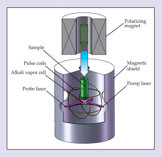
A prototypical zero-field NMR experiment is depicted schematically in figure 2. The spins are prepolarized by thermal equilibration in the field of a permanent magnet, just as in high-field NMR experiments. After polarization, the sample—assumed to be a liquid—is moved into a zero-field region inside nested layers of magnetic shielding.

Figure 2. In the zero-field experiment depicted here, the sample (green) is initially polarized in a permanent magnet and then shuttled into a magnetically shielded region (bottom). A set of coils is used to null residual magnetic fields and to apply short magnetic field pulses, which excite coherences between the nuclear spin states and set into motion spin oscillations at the sample’s J-coupling frequency. Those oscillations are detected by an atomic magnetometer, whose key component is a cell containing a vapor of alkali atoms: A pump laser polarizes the atoms, and a probe laser detects their precession, from which one can infer the magnetic field due to the sample.
Provided the sample contains at least two nuclei with distinct gyromagnetic ratios, one can put the nuclei into coherent superpositions of the singlet and triplet states by applying a short magnetic field pulse. The sample’s magnetic field then oscillates with frequency J (see the
The technique is not limited to two-spin systems; it can also be used to analyze more complex molecules. To illustrate, we show in figure 3 an experimental spectrum of acetone molecules in which both methyl groups are labeled with 13C. To understand the spectrum, first consider just one of the methyl groups. The three protons can have total spin 1⁄2 or 3⁄2. Coupling of the 13C nucleus to a combined proton spin of 1⁄2—essentially, the same problem as described above—yields a single spectral line at 1JHC ≈ 125 Hz, where the superscript indicates that one bond separates the nuclei. Coupling to a combined proton spin of 3⁄2 yields a spectral line at 2 × 1JHC ≈ 250 Hz.

Figure 3. The zero-field spectrum of acetone doubly labeled with carbon-13. (a) The molecule’s nuclear spins reside in its side methyl groups: C atoms are shown in black (with 13C indicated by asterisks), hydrogen-1 is in white, and oxygen is in red. (b) The resulting spectral pattern is uniquely determined by the J-couplings within and between the methyl groups and yields a distinct molecular “fingerprint.”
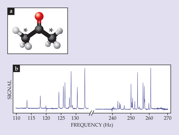
When both methyl groups are considered, one finds that the spins can be coupled through two, three, or four covalent bonds. Thus the 125- and 250-Hz lines are split, which results in the rich multiplet structure seen in figure 3b. In that way, J-coupling produces unique spectra for dozens of small molecules and provides a new, zero-field method for chemical identification.
Little fields mean a lot
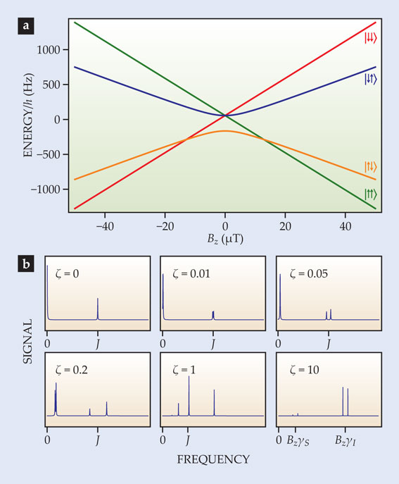
Although zero-field J-coupling spectroscopy can shed valuable light on a sample’s chemical makeup, even more information can be gleaned if a tiny, nanotesla magnetic field is applied. 10 To understand how, consider figure 4a, which shows energy levels as a function of magnetic field for a 13C–proton system with J-coupling frequency J = 220 Hz. In zero field, the triplet states are degenerate, separated in energy from the singlet state by hJ. A small field, however, lifts the degeneracy. As seen in figure 4b, the spectral line associated with the singlet-to-triplet transition splits into two, and the zero-frequency line associated with transitions between triplet states shifts upward and eventually splits. (In more complex molecules, the zero-field eigenstates span larger values of angular momentum and therefore lead to more complex splitting patterns.) When the magnetic field is sufficiently strong that the Zeeman effect is much larger than the J-coupling, the spectrum reduces to a set of two doublets, each split by J. Such near-zero-field splitting patterns can be used as a diagnostic tool to determine the types of transitions and degeneracies associated with zero-field NMR lines.

Figure 5. Parahydrogen-induced polarization can be used to obtain nuclear magnetic resonance signals in the absence of a magnetic field, as depicted here for a hypothetical three-spin system consisting of a carbon-13 nucleus and the nuclei of a parahydrogen molecule. (a) In isolation, the antiparallel spins in the parahydrogen molecule correspond to the singlet state. (b) If the molecule is catalytically added to a substrate molecule containing 13C, and if one of the C–H couplings is much stronger than the other couplings in the system, the symmetry of the parahydrogen spins is broken and in the newly formed three-spin system, the population of the upper doublet is about three times that of the lower one. (Here, we ignore the rotational energies that may be correlated with the nuclear state.) The horizontal lines represent magnetic sublevels and the red rectangles represent the expected populations in each sublevel. (c) The simulated spectrum of a system with strong C–H coupling JCH = 140 Hz, weak C–H coupling JCH = −5.2 Hz, and H–H coupling JHH = 7.7 Hz yields the three peaks shown here, which correspond to the three allowed transitions indicated by the dashed arrows in panel b.
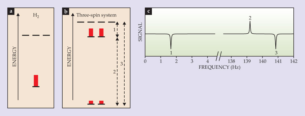

Figure 4. In a two-spin system with spins I and S, energy levels (a) and magnetic resonance spectral lines (b) shift and split as an external magnetic field Bz is applied. When the normalized magnetic field ζ = Bz(γI − γS)/J = 0, the system consists of a singlet state and degenerate triplet states; the system produces a spectral line at J corresponding to singlet-to-triplet transitions and a line at zero frequency corresponding to the static component of magnetization. (Here γ is the gyromagnetic ratio, and J is the J-coupling frequency.) As the magnetic field increases, the line at J splits into a doublet and the line at zero frequency moves to the right and eventually splits. For ζ ≫ 1, the spectrum is dominated by the Zeeman effect and consists of two doublets centered at BzγI and BzγS, each split by J. Note the change in the x-axis scale in the last two panels.
Parahydrogen-induced polarization
The spins in the previous section were polarized via thermal equilibration in a permanent magnet. However, there are several alternative means for polarizing nuclear spins, and some of them can yield polarizations much higher than one could achieve with even the strongest magnets. With dynamic nuclear polarization, for instance, spin polarization is transferred from easily polarizable electrons to nuclei by way of a process known as cross relaxation; with spin-exchange optical pumping, polarization is transferred from photons to nuclei by way of light–atom interactions and interatomic collisions. In theory, both techniques can be used to achieve nuclear spin polarizations approaching 100%; spin-exchange optical pumping is generally most effective on nuclei of noble gases such as helium-3 and xenon-129.
Recently we have begun conducting zero-field NMR experiments
8
using what is known as parahydrogen-induced polarization (PHIP).
3
Below 30 K, molecular hydrogen in equilibrium is almost exclusively parahydrogen, the nuclear spin-singlet state (∣↑↓〉 − ∣↓↑〉)/√
The parahydrogen state itself has zero magnetic moment and does not produce an NMR signal. How then can one take advantage of its high degree of spin order? The symmetry can be broken by the catalytic addition of parahydrogen to a substrate molecule containing a nonzero nuclear spin such as that of 13C or fluorine-19. Consider, for example, the reaction H2 + R=CH2 → H−R−CH3, where R is some chemical group. The parahydrogen-derived protons occupy chemically distinct sites on the product molecule and therefore have different couplings with the 13C spin.
Figures
Room to grow
Low- and zero-field NMR are best viewed as complements to traditional high-field spectroscopy and imaging. Over the years, high-field NMR has evolved into an incredibly powerful and versatile tool in research and industry, but low- and zero-field methods are likely to find important niche applications: Because they are portable, relatively inexpensive, and minimally invasive, the methods may enable mobile tools for real-time chemical analysis in microfluidic lab-on-a-chip devices. In that context, atomic magnetometers and SQUIDs might eventually give way to magnetic sensors based on nitrogen-vacancy centers in diamond. 17 Such sensors are small and highly sensitive and can operate in a broad temperature range. They’ve recently been used to measure magnetic fields generated by nanoscale samples containing just a few thousand atoms (see page 12 of this issue). In a different vein, hyperpolarized molecules undergoing J-coupling-induced quantum beats may serve as a new type of polarized target for nuclear-physics experiments. 18
Low- and zero-field NMR are still relatively young fields, and plenty of work lies ahead. In addition to the universal and perpetual challenges of boosting the sensitivity and shrinking the size of detectors, multidimensional zero-field spectroscopy techniques need to be developed to analyze the exceedingly complex spectra of biologically relevant molecules.
Origin of the zero-field signal
Consider a sample consisting of two nuclei with spins I = S = 1⁄2, polarized by a large magnetic field. Adiabatically moving the sample to zero field results in two types of nuclear spin polarization: a dipole moment in the triplet state—that is, an excess population in the ∣F = 1, MF = 1〉 = ∣↑↑〉 state relative to the ∣F = 1, MF = −1〉 = ∣↓↓〉 state—and an excess population in the singlet state ∣F = 0, MF = 0〉 relative to the ∣F = 1, MF = 0〉 state. (This can be seen by following the curves in figure 4a from high to low field.) Here, F is the total spin angular momentum and MF is its projection on the quantization axis z.
Panel a illustrates the response of the dipole polarization to a magnetic field pulse. For simplicity, we assume that all molecules start off in the state ∣↑↑〉. The effects of the applied magnetic field B are most easily understood in the uncoupled basis ∣MI, MS〉. The panel’s black and red arrows indicate the expectation values of the spin vectors I and S, both of which start off polarized in the z-direction. Assuming the spins have distinct gyromagnetic ratios γi = 2πgiμN/h—where g is the nuclear g-factor, μN is the nuclear magneton, and h is Planck’s constant—a magnetic pulse oriented in the x-direction causes the spins to rotate through different angles. For simplicity of illustration, we assume here that gI = 2gS; the ratio of the g-factors of carbon-13 nuclei and protons is roughly four to one. By tuning the duration and strength of the magnetic field pulse, we can place the spin system in the state ∣ψ(0)〉 = ∣↑↓〉 = (∣F = 1, MF = 0〉 + ∣F = 0, MF = 0〉)/√
The triplet and singlet states are separated in energy by hJ, so after the magnetic pulse, quantum beats occur between those two states at precisely the frequency J. One can show that the expectation values of the z components of the spins are 〈Iz〉 = 1⁄2 cos 2πJt and 〈Sz〉 = −1⁄2 cos 2πJt. The evolution of 〈Iz〉 and 〈Sz〉, scaled by gI and gS, is depicted by the black and red arrows, respectively, in panel b. Their sum yields the total magnetization, represented by the smooth blue curve.
The picture is only slightly different if we assume that all molecules start in the singlet state ∣F = 0, MF = 0〉 = (∣↑↓〉 − ∣↓↑〉)/√

We gratefully acknowledge support from the NSF. We also thank Alexander Pines, Max Zolotorev, Brian Patton, Bogdan Wojtsekhowski, Bernhard Blümich, Szymon Pustelny, Louis Bouchard, and Yasuhiro Shimizu for stimulating discussions and useful feedback.
References
1. D. P. Weitekamp et al., Phys. Rev. Lett. 50, 1807 (1983); https://doi.org/10.1103/PhysRevLett.50.1807
D. Zax et al., Chem. Phys. Lett. 106, 550 (1984). https://doi.org/10.1016/0009-2614(84)85381-62. T. G. Walker, W. Happer, Rev. Mod. Phys. 69, 629 (1997). https://doi.org/10.1103/RevModPhys.69.629
3. C. R. Bowers, D. P. Weitekamp, Phys. Rev. Lett. 57, 2645 (1986). https://doi.org/10.1103/PhysRevLett.57.2645
4. R. McDermott et al., Science 295, 2247 (2002). https://doi.org/10.1126/science.1069280
5. M. P. Ledbetter et al., J. Magn. Reson. 199, 25 (2009). https://doi.org/10.1016/j.jmr.2009.03.008
6. Y. S. Greenberg, Rev. Mod. Phys. 70, 175 (1998). https://doi.org/10.1103/RevModPhys.70.175
7. I. Savukov, S. Seltzer, M. Romalis, J. Magn. Reson. 185, 214 (2007). https://doi.org/10.1016/j.jmr.2006.12.012
8. T. Theis et al., Nat. Phys. 7, 571 (2011). https://doi.org/10.1038/nphys1986
9. J. Bernarding et al., J. Am. Chem. Soc. 128, 714 (2006). https://doi.org/10.1021/ja055273e
10. M. P. Ledbetter et al., Phys. Rev. Lett. 107, 107601 (2011). https://doi.org/10.1103/PhysRevLett.107.107601
11. M. Packard, R. Varian, Phys. Rev. 93, 941 (1954).
12. J. N. Robinson et al., J. Magn. Reson. 182, 343 (2006); https://doi.org/10.1016/j.jmr.2006.06.027
S. Appelt et al., Nat. Phys. 2, 105 (2006).13. S.-K. Lee et al., Appl. Phys. Lett. 89, 214106 (2006). https://doi.org/10.1063/1.2390643
14. E. L. Hahn, D. E. Maxwell, Phys. Rev. 84, 1246 (1951). https://doi.org/10.1103/PhysRev.84.1246
15. H. S. Gutowsky, D. W. McCall, C. P. Slichter, Phys. Rev. 84, 589 (1951).
16. N. F. Ramsey, E. M. Purcell, Phys. Rev. 85, 143 (1952). https://doi.org/10.1103/PhysRev.85.143
17. J. M. Taylor et al., Nat. Phys. 4, 810 (2008). https://doi.org/10.1038/nphys1075
18. D. Budker et al., Nucl. Instrum. Methods Phys. Res. A 694, 246 (2012). https://doi.org/10.1016/j.nima.2012.08.007
More about the authors
Micah Ledbetter, a physicist at AOSense Inc in Sunnyvale, California, was an assistant researcher in the department of physics at the University of California, Berkeley. Dmitry Budker is a professor in the department of physics at UC Berkeley and a faculty scientist in the nuclear science division at Lawrence Berkeley National Laboratory.


