Vegetation pattern formation: The mechanisms behind the forms
DOI: 10.1063/PT.3.4340
Mathematician Alan Turing deciphered the German Enigma code during World War II and laid the foundations of computer science as a new discipline. But toward the end of his short life, he made a lesser-known yet groundbreaking contribution. Interested in the development of patterns and shapes in biological systems, in 1952 Turing published a paper entitled “The chemical basis of morphogenesis.” 1 In the theoretical study, he showed that a homogeneous system of chemical substances that react with each other and diffuse in space can self-organize into spatially periodic distributions. His work received limited attention until four decades later, when the behavior was experimentally observed. 2 , 3 The confirmation of Turing’s prediction led to a surge in the number of studies of so-called Turing patterns, first in chemical and biological contexts and more recently in ecological contexts. 4

COURTESY OF KEVIN SANDERS
In a time when aerial photographs, let alone satellite images, of remote regions were hardly available, Turing could not have imagined the possible realizations of his predictions for dryland vegetation. Those who have traveled through arid and semiarid regions may have noticed the patchy character of the landscape, which is made up of vegetation patches surrounded by bare-soil areas or vice versa. Usually the patchiness appears irregular, which has traditionally been attributed to variable microtopography and soil heterogeneities. It came as a big surprise when aerial photographs of dryland regions, first in East Africa 5 (even before Turing’s paper) and later in many regions across the world, revealed strikingly regular vegetation patterns with various morphologies that were not recognizable from the ground.
The first morphology to receive extensive scientific attention was parallel vegetation bands on gently sloped terrains,
6–8
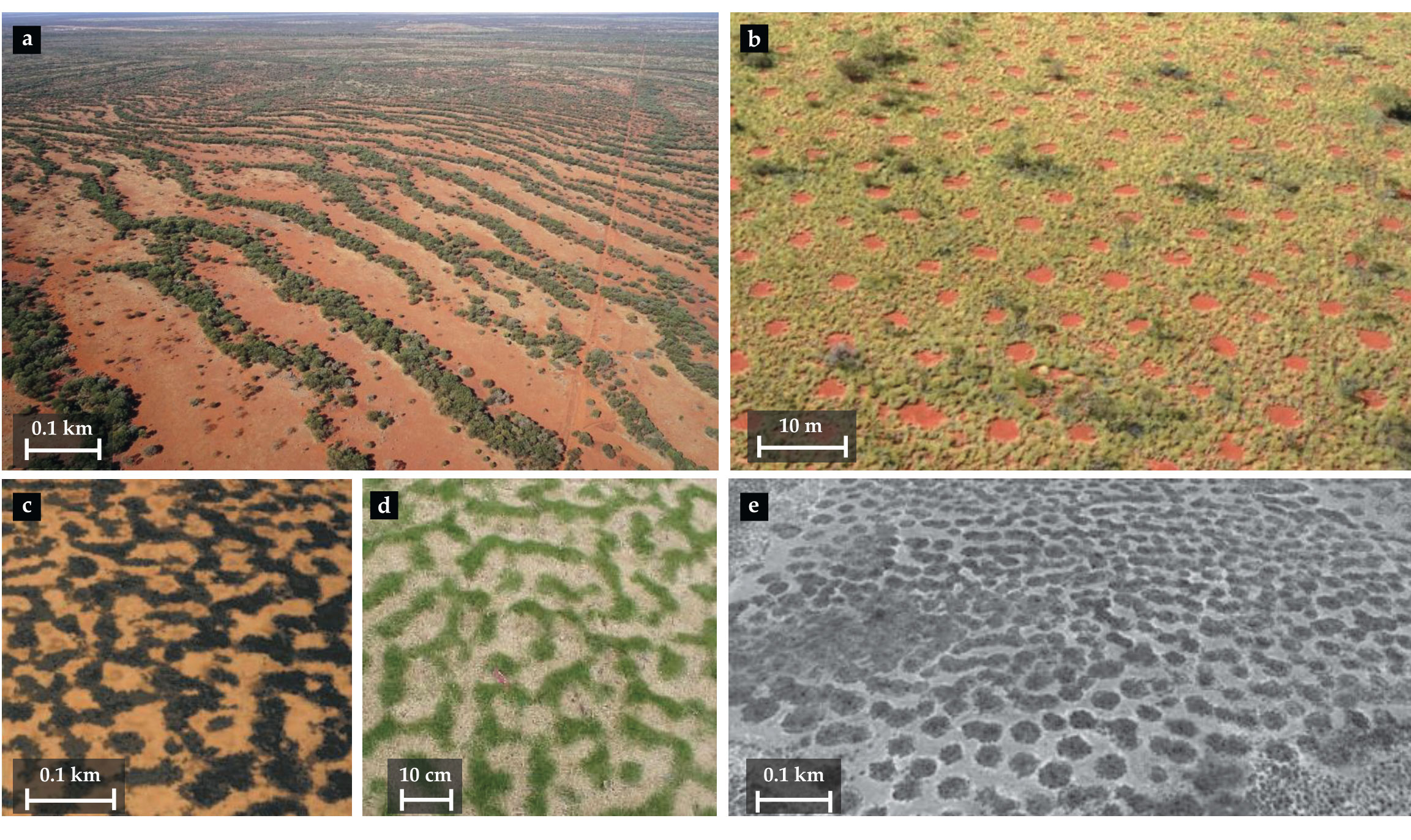
a recent example of which was observed in northwestern Australia (see figure
Figure 1.

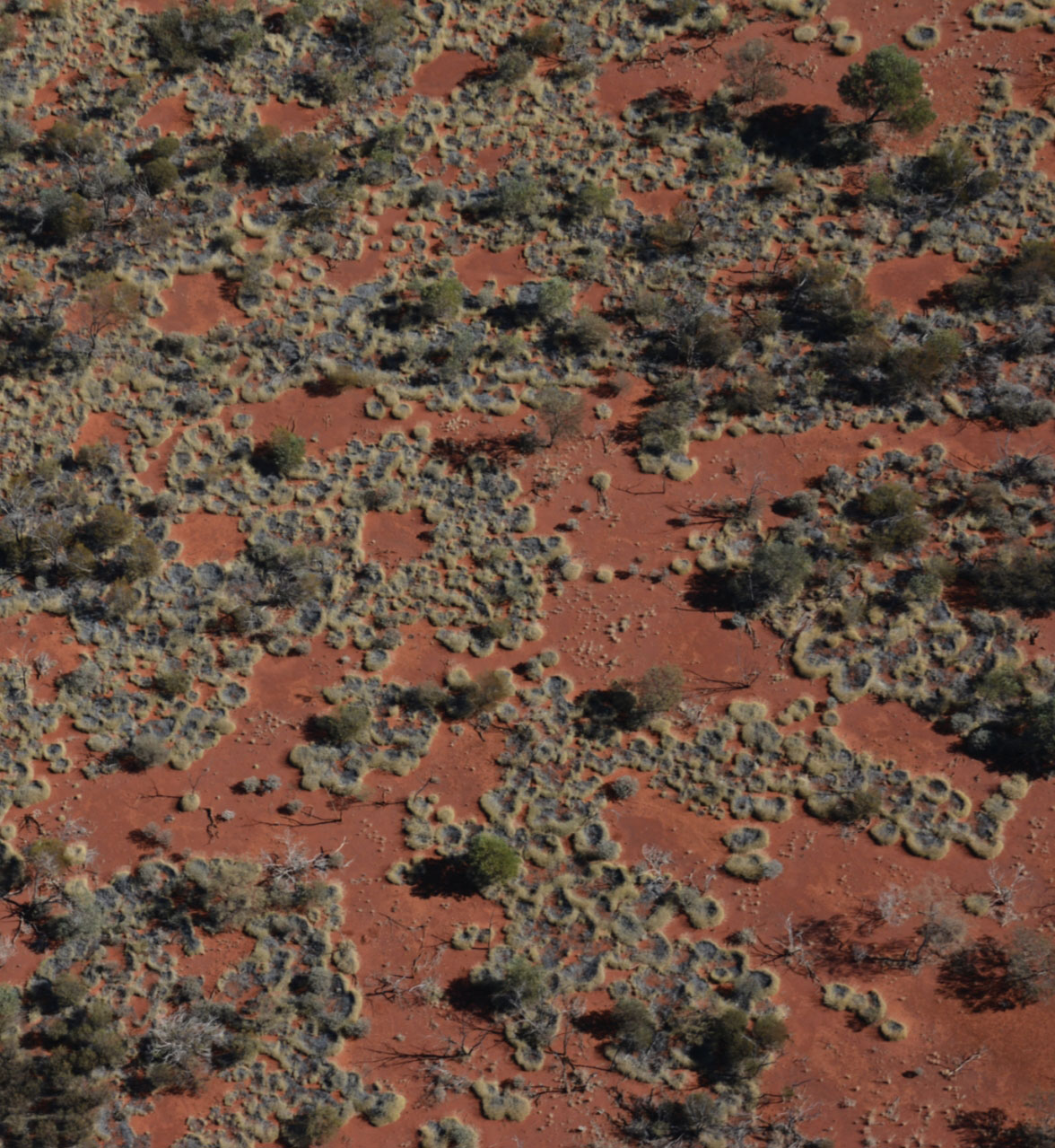
Dryland vegetation can form a range of patterns. (a) Banded woody vegetation on a sloped terrain in Australia (photo courtesy of Stephan Getzin). (b) A gap pattern of herbaceous vegetation in Australia (from ref.
Vegetation patterns are not limited to drylands. 4 Recently they have also been observed in underwater seagrass maps obtained using hydroacoustic techniques. 9 The growing recognition of vegetation pattern formation as a fundamental phenomenon observed worldwide with different plant species has led to the emergence of a vigorous new research field at the interface between spatial ecology, nonlinear physics, and applied mathematics, 10 where Turing’s ideas are essential.
Positive water–biomass feedback
The spontaneous appearance of large-scale spatial order is often a result of a local positive feedback loop that amplifies small perturbations throughout the whole system and thereby induces an instability of the original state. But what positive feedback loop could drive the formation of the observed periodic vegetation patterns? Assuming that pattern formation in water-limited ecosystems can be explained solely in terms of vegetation growth and water availability, researchers have proposed a feedback loop, illustrated in figure
Figure 2.

A positive feedback loop drives vegetation pattern formation in water-limited systems. Feedback mechanisms accelerate vegetation growth in denser patches and inhibit growth in adjacent sparser patches, and thereby promote vegetation pattern formation. (Adapted from ref.
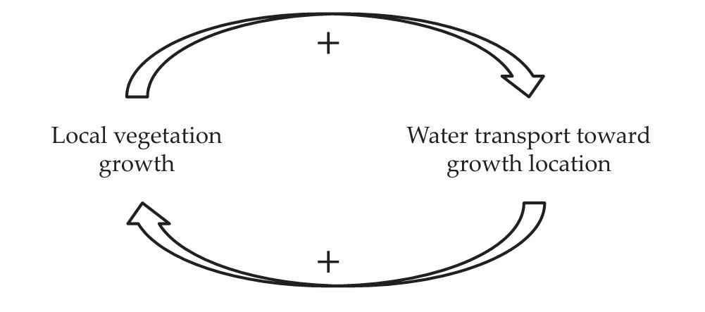
An instability driving uniform vegetation to become patterned can then be understood as follows: Consider a landscape of almost uniform vegetation and an area with slightly denser vegetation than its surroundings. That area draws slightly more water than its surroundings and becomes even denser. The amplified deviation from the originally uniform vegetation closes the feedback loop and sets the ground for a new amplification loop. While the transport of water toward denser vegetation accelerates the growth there, it inhibits the growth in the surrounding areas from which water is being taken. The instability that results generates nonuniform vegetation growth and the formation of a pattern. 4
The first part of the feedback loop (the lower arrow in figure
One possible process is overland water flow, shown in figure
Figure 3.

Three forms of water transport promote flow toward vegetation patches. (a) Overland water flow is induced by differences in water infiltration, which is low in bare-soil areas covered by soil crusts, indicated here by a thick ground-surface line, and high in vegetated areas. (b) Laterally extended root systems allow plants to increase their water uptake by drawing from a larger volume. (c) Water diffuses from water-rich soil in nonvegetated areas with high infiltration rates to water-poor soil in vegetated areas. Dark-blue arrows denote water transport toward growing vegetation. Short light-blue arrows denote low surface-water infiltration rates, and long light-blue arrows denote high infiltration rates. Shaded blue in the soil denotes high water content.
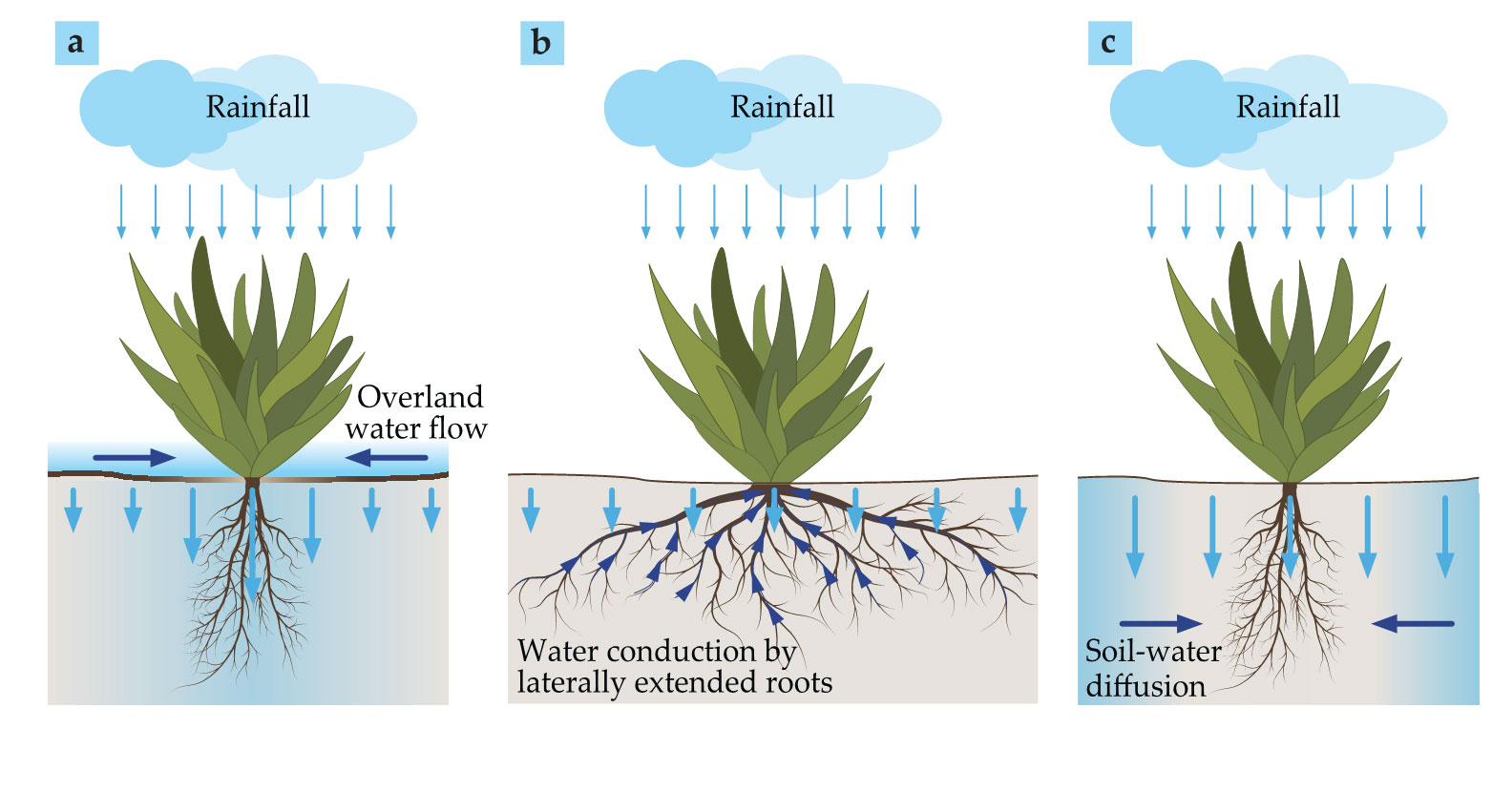
Another mechanism is conduction by laterally extended plant roots (see figure
The root-to-shoot relationship also is essential in enhancing water transport for laterally confined roots (see figure
The three mechanisms are each associated with a positive feedback loop that can induce a pattern-forming instability on its own. In general, the feedback loops can act in concert, and their relative importance changes with environmental conditions. The interplay between them has interesting implications for community structures because of the different water distributions associated with each transport mechanism and the niches those distributions provide for other species. 10 , 11 The feedback loop associated with overland water flow acts to increase the soil-water content in a vegetation patch, whereas those loops associated with water diffusion and conduction by lateral roots act to decrease that content by their strong water uptake. In landscapes consisting of shrubs and annual plants, dominance of the overland water flow feedback loop can facilitate annuals growing near or under the canopies of shrubs; dominance instead of feedback loops involving strong water uptake can result in the exclusion of annuals from the vicinities of shrubs. 11 , 12
Upscaling information from local to global
The biomass–water feedback loops describe local plant-scale processes. But does that small-scale information translate to large-scale collective behaviors? Specifically, can the capabilities of the biomass–water feedback loops induce pattern-forming instabilities in uniform vegetation?
One indispensable tool for addressing such questions is a heuristic mathematical model, built so as to capture the feedback loops associated with overland water flow, water conduction by laterally extended roots, and water transport by diffusion.
Two types of modeling approaches are primarily used to study plant population dynamics: discrete agent-based models, also called individual-based models, and those based on continuum partial differential equations (PDEs). Agent-based models are stochastic computational algorithms that go down to the level of individual plants and often describe each plant in great detail. PDE models, on the other hand, do not address individual plants; rather, they describe deterministic processes at small spatial scales. A plant population is then represented by a continuous biomass areal density.
The PDE approach is more heuristic but has the advantage of lending itself to the powerful methods of pattern-formation theory. 10 But is it a suitable approach to describe small populations of discrete entities, for which demographic noise and extinction are usually a concern? The answer is definitely positive. Unlike animals, plants are immobile organisms that cannot migrate away from environmental stresses. Instead, they generally cope by changing their phenotype. That plasticity is reflected in, among other things, the ability of a single plant to change its viable biomass by orders of magnitude; such flexibility justifies embodying vegetation biomass as a continuous variable. Another consideration that supports the continuum modeling approach is the near irrelevance of extinction events; even in cases of complete plant mortality, long-lived seeds have nonvanishing probabilities of germinating whenever the biotic and abiotic conditions allow and can revive the population.
In 2004 Erez Gilad and colleagues introduced a PDE model that captures all three feedback loops.
12
It contains a biomass variable
The positive feedback loop associated with laterally extended roots is captured by making the width of the localized root kernel
Applications of the general model to specific ecological contexts often allow simplifications. For example, a model for species with confined root zones can be simplified by using delta-function root kernels; that assumption results in the replacement of the nonlocal integral terms by local algebraic functions. A model for ecosystems with sandy soil characterized by high infiltration rates can be simplified by eliminating the overland-water equation. 10
PDE models of dryland ecosystems often oversimplify the complex ecological reality and leave aside many factors, such as the effect of transpiration on the atmosphere, soil erosion and deposition, and various plant-physiology processes. They should be viewed as tools that can provide deep insights into given ecological contexts rather than make quantitative forecasts. The models also constitute an indispensable source of well-grounded hypotheses for empirical studies. Such studies are typically long running because of the time scales on which vegetation grows; the hypotheses being tested should therefore be carefully chosen.
Emergence of large-scale periodicity
Analytical and numerical studies of the model discussed above have shown that all three biomass–water feedback loops can induce a nonuniform stationary instability of uniform vegetation when the precipitation rate
A convenient way to graphically describe the model solutions and show their existence and stability ranges is to draw a bifurcation diagram such as the one in figure
Figure 4.

Periodic and localized patterns emerge from a nonuniform instability of uniform vegetation. (a) A bifurcation diagram of one-dimensional solutions of a two-variable model that shows the dependence of the
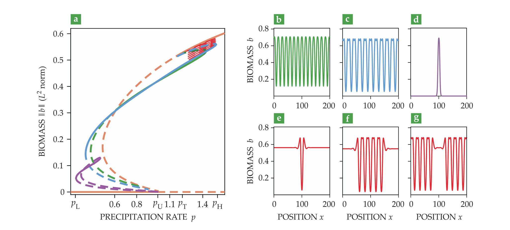
Figure
In addition to the periodic solution that emerges from the uniform vegetation solution branch at
The green and blue periodic-solution branches that emerge from the uniform vegetation solution appear in subcritical bifurcations—that is, a precipitation range exists where both uniform vegetation and periodic patterns are stable states. That range extends from the threshold
Within that range there exist a multiplicity of stable localized patterns of increasing size, beginning with a gap in otherwise uniform vegetation (figure
In two-dimensional isotropic systems, nonuniform stationary instabilities generally result in the emergence of periodic hexagonal patterns. Such patterns are formed by the simultaneous growth of three resonant modes with wavevectors of the same magnitude
Figure 5.

The five basic vegetation patterns along the rainfall gradient (green panels) and snapshots of two morphological transitions (black-and-white panels) as obtained by model simulations with slowly decreasing rates of precipitation. As precipitation decreases from left to right, bare-soil areas, which contribute water to adjacent vegetation areas, should increase in size for the vegetation to remain viable. That increase results in two morphological transitions: Gaps become stripes through the merging of bare-soil gaps, and as vegetation disintegrates further, those stripes turn into spots.
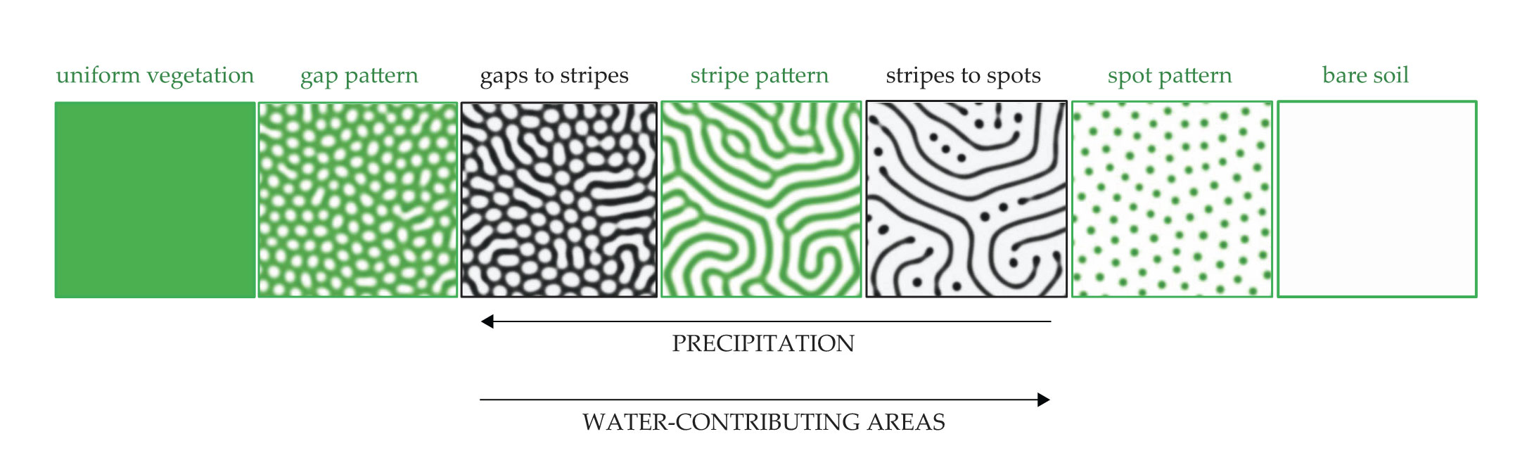
Ecosystems with sloped terrains are not isotropic, and the patterns that emerge from simulations are mostly stripes oriented perpendicular to the slope. That finding is consistent with empirical observations,
8
such as the stripes in figure
A basic principle for vegetation patterning
The emergence of periodic patterns from uniform vegetation as the rate of precipitation decreases can be viewed as a population-level mechanism—one that involves many individual plants—to cope with the water stress caused by reduced rainfall. Partial plant mortality and the concomitant formation of bare-soil gaps create an additional water source for the surrounding vegetation through the various forms of water transport illustrated in figure
The simplest mechanism by which bare-soil areas can increase is by a contraction of vegetation patches. In one-dimensional patterns, such as banded vegetation on sloped terrains, that contraction amounts to vegetation bands narrowing while their number stays constant, which keeps the pattern’s wavenumber unchanged. That response mechanism occurs along the branch of any periodic solution, such as the green and blue lines in figure
Two-dimensional patterns have yet another mechanism for increasing bare-soil area in response to decreasing rainfall: the morphological transitions illustrated by the black-and-white panels in figure
From patterns to function
The discussion so far has focused on understanding mechanisms of vegetation pattern formation and accounting for the variety of patterns observed in drylands. But beyond the obvious curiosity raised by those fascinating phenomena, there are important open questions related to functional aspects of vegetation patterning that call for further study. The functioning of dryland ecosystems is currently threatened by two main factors. The first is global climate change and the likely more frequent extremes, such as severe droughts, that accompany it; the second is human intervention, which often involves extracting resources, such as livestock feeding, and imposes additional stresses on already vulnerable ecosystems.
Climate extremes can cause abrupt and irreversible transitions in vegetation that lead to alternative dysfunctional stable states, such as bare soil. How do the many stable vegetation pattern states affect such transitions? Can they mitigate the effects of extreme droughts by providing alternative vegetation response pathways that culminate in functional patterned states rather than collapse to bare soil?
Human intervention also often results in detrimental outcomes. But whereas researchers need to understand the many stable ecosystem states to address the effects of climate extremes, they have to study unstable ecosystem states to deal with human intervention. Directions in which an ecosystem departs from its unstable states can act as road signs for judicious human interventions. Following those signs may circumvent detrimental outcomes by directing ecosystems toward functional states. However, identifying the relevant unstable states for particular human interventions remains a challenge.
Understanding the transient dynamics of dryland ecosystems caused by climate extremes and human intervention calls for interdisciplinary collaborations between physicists, applied mathematicians, and ecologists. By working together, they can assimilate the concepts and methodologies of pattern formation into ecological theories and facilitate research progress.
References
1. A. Turing, Philos. Trans. R. Soc. Lond. B 237, 37 (1952). https://doi.org/10.1098/rstb.1952.0012
2. V. Castets et al., Phys. Rev. Lett. 64, 2953 (1990). https://doi.org/10.1103/PhysRevLett.64.2953
3. Q. Ouyang, H. Swinney, Nature 352, 610 (1991). https://doi.org/10.1038/352610a0
4. M. Rietkerk, J. van de Koppel, Trends Ecol. Evol. 23, 169 (2008). https://doi.org/10.1016/j.tree.2007.10.013
5. W. Macfadyen, Geogr. J. 116, 199 (1950). https://doi.org/10.2307/1789384
6. R. Lefever, O. Lejeune, Bull. Math. Biol. 59, 263 (1997). https://doi.org/10.1007/BF02462004
7. C. Klausmeier, Science 284, 1826 (1999). https://doi.org/10.1126/science.284.5421.1826
8. V. Deblauwe et al., Ecol. Monogr. 82, 3 (2012). https://doi.org/10.1890/11-0362.1
9. D. Ruiz-Reynés et al., Sci. Adv. 3, e1603262 (2017). https://doi.org/10.1126/sciadv.1603262
10. E. Meron, Nonlinear Physics of Ecosystems, CRC Press/Taylor & Francis (2015).
11. E. Meron, Annu. Rev. Condens. Matter Phys. 9, 79 (2018). https://doi.org/10.1146/annurev-conmatphys-033117-053959
12. E. Gilad et al., Phys. Rev. Lett. 93, 098105 (2004). https://doi.org/10.1103/PhysRevLett.93.098105
13. R. Bastiaansen et al., Proc. Natl. Acad. Sci. USA 115, 11256 (2018). https://doi.org/10.1073/pnas.1804771115
14. E. Knobloch, Annu. Rev. Condens. Matter Phys. 6, 325 (2015). https://doi.org/10.1146/annurev-conmatphys-031214-014514
15. Y. R. Zelnik, E. Meron, G. Bel, Proc. Natl. Acad. Sci. USA 112, 12327 (2015). https://doi.org/10.1073/pnas.1504289112
16. S. Getzin et al., Proc. Natl. Acad. Sci. USA 113, 3551 (2016). https://doi.org/10.1073/pnas.1522130113
17. J. A. Sherratt, J. Math. Biol. 51, 183 (2005). https://doi.org/10.1007/s00285-005-0319-5
18. F. Borgogno et al., Rev. Geophys. 47, RG1005 (2009). https://doi.org/10.1029/2007RG000256
More about the authors
Ehud Meron is a professor of physics and the Phyllis and Kurt Kilstock Chair in Environmental Physics of Arid Zones in the Jacob Blaustein Institutes for Desert Research at Ben-Gurion University of the Negev in Israel.


