Thermochronology and landscape evolution
DOI: 10.1063/1.3226750
Mountain ranges and other large-scale features of Earth’s surface set basic patterns of climate, ecology, hydrology, and even culture. Most of us view such features as static geographic boundary conditions or possibly as monuments to some esoteric episode of ancient Earth history. But over geologic time scales, mountains and landscapes are as dynamic and ephemeral as clouds, piling up and rising, deforming, and dissipating over space and time. Just as clouds manifest the influence of the surface on atmospheric processes such as air convection, so landscapes express how the surface affects dynamic deep-Earth processes such as mantle convection.
Most landscape evolution involves deformation of Earth’s lithosphere—the crust and upper mantle, typically about 100 km thick—and erosion of its surface. In regions where tectonic plates converge, for example, faults or other localized crustal deformation can drive bedrock upward relative to some suitably fixed datum such as sea level. That, in turn, leads to surface uplift. As the surface rises, the weight of the locally supported topography increases. That increasing weight inhibits further rock uplift unless material is removed from the surface by erosion and transported somewhere else.
Erosion is limited by the supply of water on the surface and the force of that water—be it liquid or solid, as in the case of glaciers—as it flows downhill. Generally, uplifted surface topography has more of each, for two reasons. First, when air is forced to flow over an uplifted surface, precipitation tends to increase. Second, the margins of uplifted surfaces typically have steep slopes; as a result, water flowing downhill exerts a relatively large shear stress and has an enhanced carrying capacity. The couplings among rock and surface uplift, erosion, and the processes that generate increased precipitation and slope have attracted much interest from geologists. Not only do they govern how landscapes evolve, they also reveal the landscape as a dynamic link between lithospheric and atmospheric processes.
Time–temperature histories
To understand the evolution of landscapes and the broader implications of their dynamics, one might begin with simple questions: How long has a mountain range had the form we see today? Is its relief increasing or decreasing over time? How old is a canyon? Is it cutting into bedrock? What are the spatial patterns of rock uplift and surface uplift in tectonically active regions? How do those uplifts relate to patterns of rainfall, river drainage, and tectonic faults? Do the synergies among uplift, precipitation, and erosion act to localize deformation in certain regions, producing so-called crustal aneurysms?
Addressing such questions requires an understanding of spatial and temporal patterns of rock movement relative to Earth’s surface. Exhumation, the relative movement of rocks toward the surface, occurs by several mechanisms. In the context of landscape evolution, the most important is erosion.
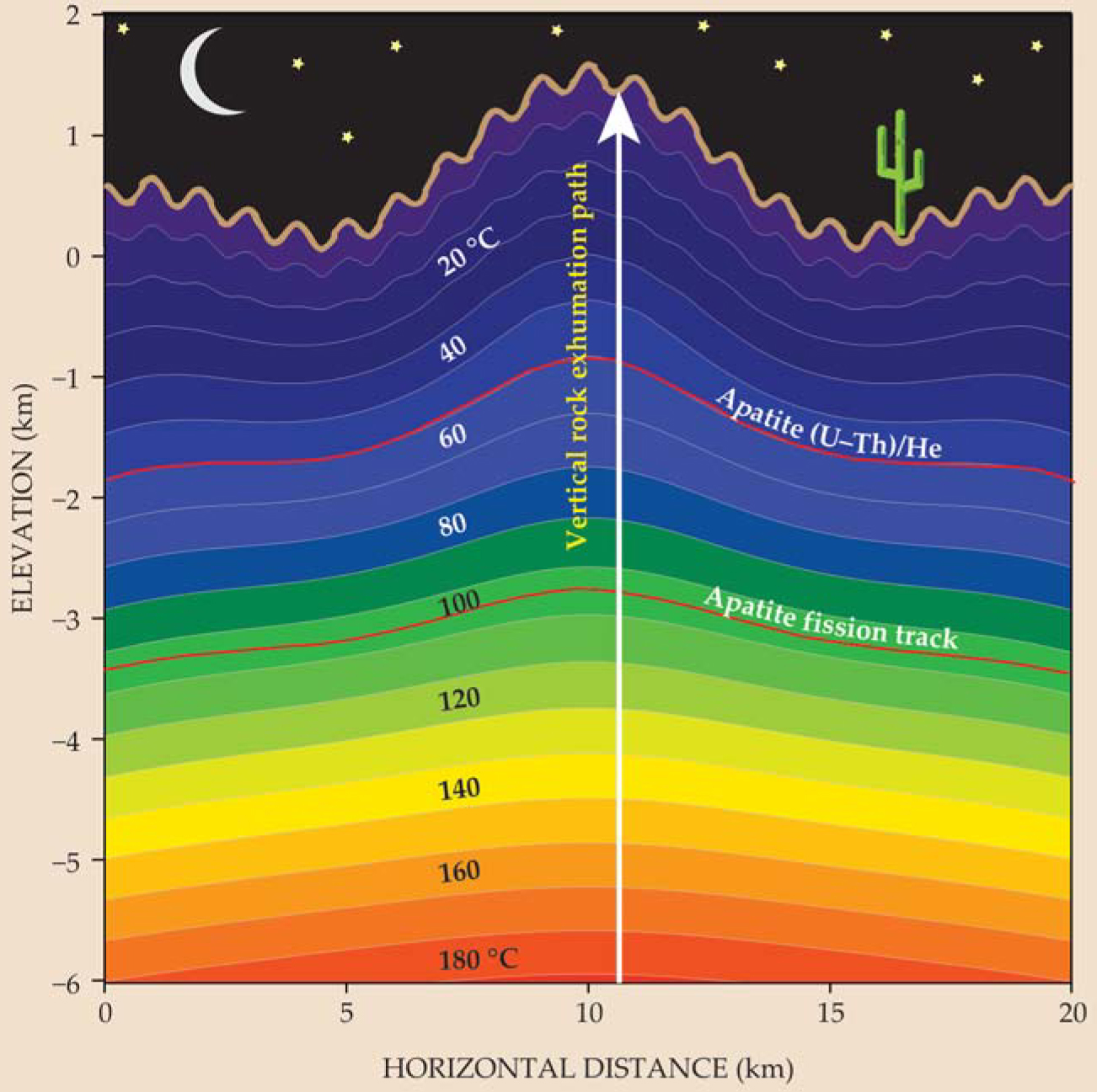
One way to measure erosion is with cosmogenic nuclides formed at known rates in rocks by incident cosmic radiation. The characteristic penetration depth of cosmic rays, however, is only a few meters. Thus cosmogenic nuclides provide a snapshot of processes acting over relatively short time frames—the time it takes for rocks to be exhumed through the affected depth, typically 1000 to 10 000 years in most techtonically active regions. By comparison, most tectonic and surface processes that interact to modify the large-scale dynamics of mountain ranges take place over a period of 105–107 years. To get a handle on those processes, one can exploit the reasonably reliable temperature profile in the conductive cooling boundary layer of the upper 10 km or so of Earth’s crust, shown in figure 1. As rocks are exhumed through the thermal field, they cool—ultimately to ambient surface temperatures. Time-versus-temperature (t–T) histories of exhumed rocks therefore provide estimates of the timing and rate of exhumation.

Figure 1. A temperature-versus-depth profile helps determine the history of rocks exhumed to Earth’s surface. Shown here are model isotherms (contours of constant temperature) beneath a simple periodic topography with three component wavelengths. Beneath the surface (brown contour), temperature increases with depth at a rate of about 20–30 °C/km, so as a rock is exhumed toward the surface, it cools. Thermochronometers provide time-versus-temperature histories of rocks. Together with some knowledge of subsurface thermal fields, such as the thermal profile shown here, they yield the timing and rate of exhumation. Because the surface topography influences the details of the subsurface thermal field, thermochronometers can sometimes be used for estimating the form of paleotopographic features. The red contours give so-called closure temperatures T c of two commonly used thermochronometers in the mineral apatite that are discussed in the text.
One of the most direct ways to establish t–T histories is with thermochronology, a technique that takes account of both the growth of daughter products—nuclides or crystallographic damage tracks—from radioactive decay and the temperature-dependent diffusive loss or annealing of those daughters. Thermochronology has a long history of use in Earth and planetary sciences. It has been applied to wildfires and meteorite histories and to a number of phenomena involving temperature change including hydrothermal fluid flow (for example, the movement of hot water in Earth’s crust), fault motion, and planetary impacts. Its most useful role in tectonics and geomorphology may be its ability to constrain t–T histories and so shed light on exhumation. The spatial and temporal patterns of exhumation, in turn, provide constraints on rates and mechanisms of landscape evolution and the tectonic forces and surface processes that control them.
In the past few decades, improvements in analytical and interpretational techniques have advanced Earth and planetary scientists’ understanding of thermochronometers and how they can be applied to study Earth and planetary processes. In this article we highlight some of the radioisotopic and kinetic foundations of thermochronology, sketch some modern analytical and interpretational approaches, and present several examples.
Thermochronology basics
As suggested above, one part of thermochronology involves the measurement of daughter products and the parent nuclides whose decay generated them. Parent and daughter product abundances are related to time through the radioactive decay equation, which follows rate laws laid out by Ernest Rutherford and others at the beginning of the last century: d = d 0 + N (eλt − 1). Here d and d 0 are the number of daughter nuclides or damage tracks now and at time t in the past, respectively; N is the number of parent nuclides now; and λ is the decay constant of the parent nuclide—that is, λdt is the probability for a nuclide to decay in an infinitesimal time dt. For thermochronological applications, d 0 is often negligible; the abundance of daughter nuclides solely reflects nuclear decay that takes place after the mineral forms.
Most thermochronological systems used in tectonic geomorphology involve one of three decay systems in several different types of minerals. The first, called the (U–Th)/He system, primarily involves production of helium-4 from the alpha decay of uranium-238, uranium-235, thorium-232, and their intermediate daughters. In the second system, crystallographic damage zones called fission tracks are produced by relatively rare but energetic spontaneous fission of 238U. The last of the three, the K–Ar system, yields argon-40 by electron capture from potassium-40. Only about 11% of 40K decays to 40Ar; the rest decays to calcium-40 by β emission.
Minerals most commonly used for thermochronology contain parts per million to percent concentrations of the parent nuclides. They include apatite [Ca5(PO4)3(F,Cl)] and zircon (ZrSiO4) for the (U–Th)/He and fission-track systems, and feldspars (calcium-, iron-, and magnesium-bearing aluminosilicates) and micas, including biotite and muscovite (silicate minerals rich in iron and magnesium), for the K–Ar system.
If daughters were not lost over time, their growth would follow the radioactive decay equation, or a slightly modified form for the branched decay of 40K. However, what distinguishes thermochronological systems from conventional geochronological systems is that daughter nuclides can be lost through diffusion and damage tracks can be wiped out through annealing. Thus inserting into the radioactive decay equation the measured values of parent nuclides and daughter products in a mineral will give a thermochronological age (“age” for short) that is less than or equal to the formation age of the mineral. Minerals that cooled slowly or that were recently reheated can have thermochronological ages that are much less than their formation ages.
A quantitative interpretation of thermochronological ages thus requires an understanding of the kinetics of diffusion or annealing of daughter products in host minerals. In that regard, controlled laboratory experiments provide essential data. A fundamental assumption is that the kinetics observed in laboratory conditions and time scales applies in natural conditions and over much longer time scales. Experiments show that diffusive loss of He and Ar from minerals can be well described by the Arrhenius law
Here D is the diffusion coefficient; D 0 is its value in the limit of infinite temperature; Ea is the molar activation energy appropriate to the diffusing process; a is the characteristic length scale of the diffusion domain, typically the size of the crystal or mineral grain itself; R is the gas constant; and T is absolute temperature. In practice, one typically measures D/a 2. Indeed, that quotient is the parameter that controls the amount of daughter loss as a function of t and T; for a given D, a small crystal or grain will lose daughters faster than a large one. The annealing of fission tracks is a more complex process than the diffusion of noble gases and for most applications is described in terms of experimentally derived parameters fit to a kinetic model.
In nature, the temperature and therefore the rate of diffusion controlling daughter loss from a mineral will vary. Over geologic time the system might undergo some periods of high temperature, during which it experiences significant diffusive loss. At other times, when the temperature is sufficiently low, daughter products are completely retained within the mineral.
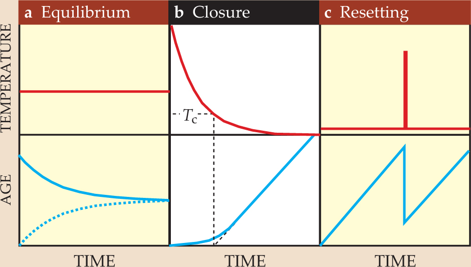
Figure 2 illustrates how thermochronological age varies with time for three specific types of thermal histories. First, consider a mineral held at constant temperature for a long period of time. Regardless of the thermochronometer’s initial daughter concentration, a thermochronometer approaches an equilibrium age at which the daughter product concentration represents a balance of radiogenic production and diffusive loss. Next, consider a mineral that experiences a monotonic temperature change from high to low—for example, as it is exhumed toward the surface by erosion. In that case, the thermochronological system passes through a known closure temperature Tc that depends primarily on the diffusion kinetics of the system. Figure 1, for example, indicates Tc for exhuming apatite (U–Th)/He and fission-track systems. Once the sample has cooled significantly below Tc , essentially all daughter products are retained. In that monotonic cooling context—the context in which thermochronological ages are often interpreted—Tc may be defined so that a sample’s age is the time elapsed since cooling below Tc. Finally, a sample held at a low temperature for a period of time may experience a reheating event that leads to high diffusivity and partial loss of daughter product. In that case, its age will be reset to a lower value.

Figure 2. Thermochronological age is determined by comparing the amount of parent nuclide and daughter product in a mineral. Temperature affects the rate at which daughter products are lost, so age evolution reflects temperature evolution. (a) Given enough time, a system held at a constant temperature will reach an equilibrium age independent of the initial daughter concentration (solid and dashed curves). (b) When a system cools from high to low temperature, it passes through a closure temperature Tc below which essentially no daughter product is lost. As shown graphically, T c may be defined so that the thermochronological age equals the time since passage through T c. (c) A brief period of high temperature can cause the loss of daughter nuclides; as a result, the thermochronological age is reset to a lower value.
Obviously, the thermal histories of real rocks are more complex than those illustrated in figure 2. Natural histories may involve multiple phases of closure, resetting, and approach to equilibrium age. In general, it’s no simple matter to determine the t–T histories that are consistent with observed thermochronological ages; indeed, doing so represents much of the geologic and computational interpretation involved in thermochronology. Nonetheless, in many cases, and especially in tectonically active landscapes, the assumption of monotonic cooling is well justified and provides a great deal of interpretive power.
How to read a thermochronometer
Thermochronometry begins with the determination of a parent-daughter ratio in a mineral. Daughters He and Ar, in particular, are readily released by heating and measured by gas-source mass spectrometry. Measurement of the parent nuclides U, Th, and K requires chemical isolation followed by, for example, atomic absorption spectroscopy or inductively coupled plasma mass spectrometry. For a fission-track sample, one counts the daughter damage tracks on an exposed internal crystal surface that has been chemically etched to make the tracks visible and measures the amount of parent 238U in the same sample.
The (U–Th)/He, fission-track, and K–Ar systems usually contain potentially useful clues that reveal more of the t–T history than just a single age and temperature. For example, although different specimens of the same type of mineral have similar diffusion or annealing kinetics, they also have natural differences in grain-size distribution, composition, radiation damage, and other properties. Those natural variations can cause differing rates of daughter product loss, and therefore age, even among grains from the same rock. With suitable analysis, those differences can be used to constrain t–T paths.
For noble gas systems, another powerful constraint on thermal histories is the spatial distribution of daughter products within a crystal. Figure 3 illustrates the idea. In brief, a uniform core-to-rim concentration means that the sample experienced insignificant diffusive loss as it cooled and thus indicates that the cooling was rapid. By contrast, a decreasing core-to-rim daughter concentration requires either a reheating event or prolonged residence at temperatures where the daughter nuclides are only partially retained; the latter scenario indicates slow cooling.

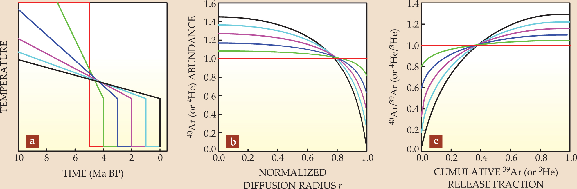
Figure 3. Distributions of daughter nuclides constrain time–temperature histories. (a) The six cooling histories shown here would yield identical (U–Th)/He or K–Ar ages of 5 million years. The time on the axis is given in millions of years before the present. (b) Each t–T history implies a color-matched spatial distribution of daughter nuclides (argon-40 or helium-4) across a spherical diffusion domain. The integrals of these abundance curves over volume yield equal 40Ar or 4He abundances, consistent with the common age of the six systems. The abundances are given in arbitrary units and the radial coordinate r is normalized so that the edge of the domain is at r = 1. The t–T history in panel a with the instantaneous drop (orange) corresponds to a uniform spatial distribution. Spatial gradients are more pronounced as the cooling slows. (c) What is actually measured is the ratio of 40Ar to 39Ar (or 4He to 3He) as they are released during sequential heating experiments. Each ratio plot corresponds to the same-colored thermal history in panel a.
In some cases intracrystalline daughter-product concentration gradients can be measured directly by analyzing small pits ablated by short-wavelength lasers. In practice, however, they are typically measured indirectly. One diffuses out small aliquots of gas originating from progressively greater depths in the crystal and compares natural daughter isotopes (4He or 40Ar) with synthetic isotopes that are simultaneously diffused from the sample during controlled heating. For the (U–Th)/He system, one creates a uniform distribution of 3He in the minerals by bombarding it with high-energy protons. Variations in the 4He/3He ratios extracted in sequential heating steps then reflect the intracrystalline concentration profile of 4He.
A similar approach works for the K–Ar system. Prior to analysis, one irradiates a sample with energetic neutrons, converting some of the 39K in the sample to 39Ar. The 40Ar/39Ar ratios in aliquots released in a step-heating experiment reveal the intracrystalline concentration profile of 40Ar. For that system, each individual gas aliquot also yields an age, because the 39Ar is produced directly from 39K and the natural 40K/39K ratio is known. By contrast, the uniformly produced 3He in the (U–Th)/He system is unrelated to the parent nuclides, though it does provide an indication of the natural 4He distribution.
Applications to rock uplift and erosion
Most mountainous topography is found near boundaries of tectonic plates. At depths down to 10-15 km, faulting in brittle rocks is largely responsible for crustal deformation; at greater depth and higher temperature, deformation occurs principally via the ductile flow of rock. Spatial gradients in rock uplift, in turn, lead to nonuniformities in surface uplift and its associated erosion. From a different perspective, one sees that spatial patterns of both surface elevation and erosion reflect the large-scale forces causing crustal deformation. One of the most powerful roles of thermochronology is to use thermochronological ages to estimate erosion rates over landscapes; often the patterns they reveal provide surprising insights into crustal deformation that are not readily deduced from the topography itself.
As its long-time residents know from the frequent earthquakes they experience, Southern California is tectonically active. A large part of the region is a transform plate boundary at which the San Andreas fault accommodates lateral motion of the Pacific and North American plates. Such purely lateral motion doesn’t usually cause much rock uplift, but northeast of Los Angeles, the orientation of the San Andreas fault changes; the resulting broad region of complex and locally compressive strain created and continues to shape the rugged San Bernardino and San Gabriel mountain ranges. By analyzing spatial patterns in the ages of (U–Th)/He and fission-track thermochronometers found throughout those ranges, Virginia Tech geologist James Spotila has produced erosion rate maps (see figure 4) that elucidate the underlying patterns of rock uplift.

Figure 4. Erosion rates vary by two orders of magnitude in the San Bernardino Mountains astride the San Andreas fault (black) in Southern California. Cited erosion rates are based on (U–Th)/He and fission-track age patterns in the mineral apatite and supported by other observations, including cosmogenic nuclide abundances and geomorphic data such as the extent of weathering and the steepness of streams. Arrows indicate the relative motion of blocks on either side of the fault.
(Adapted from J. A. Spotila
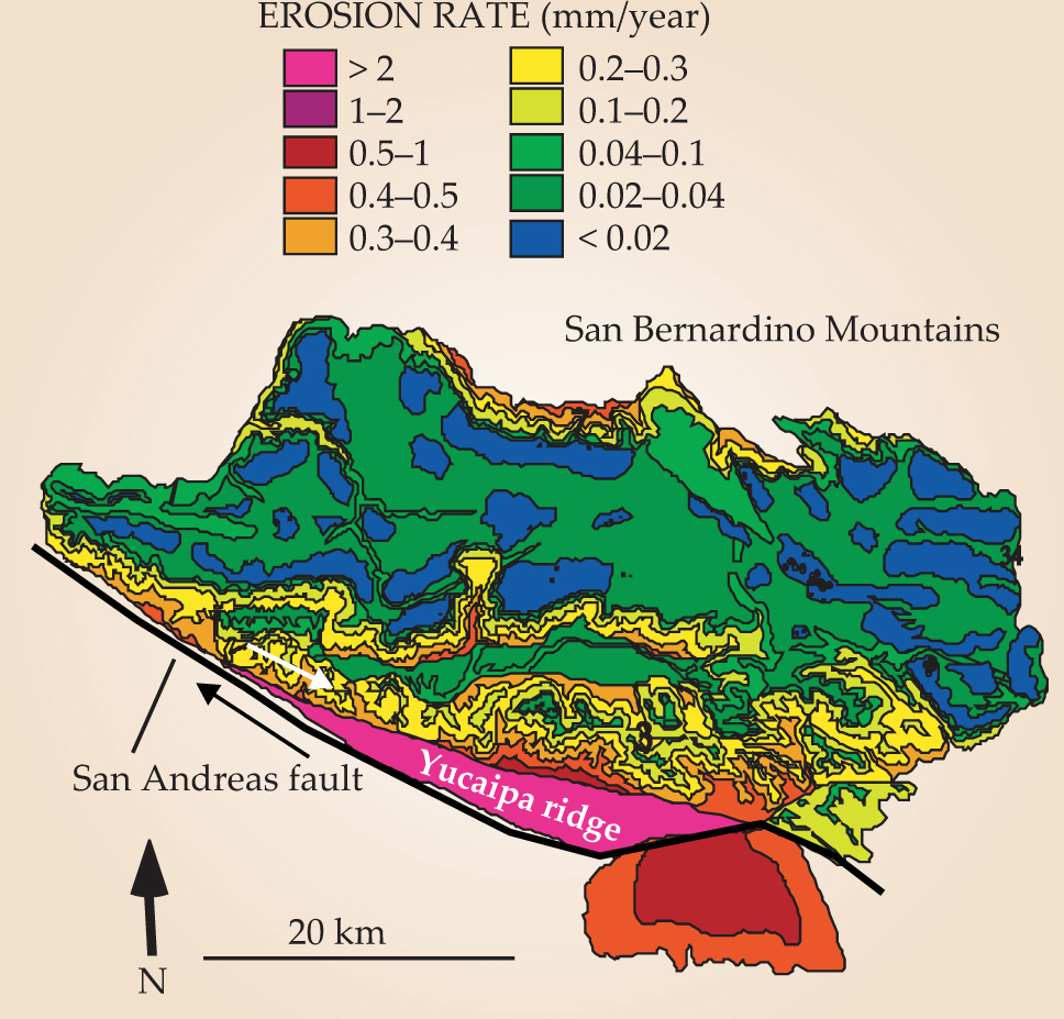
In general, uplift rates decrease away from the San Andreas fault, but deformation partitions into blocks. In the San Bernardinos, rocks in the so-called Yucaipa ridge, a 5-km-wide block adjacent to the fault, have apatite (U–Th)/He ages of 1 to 2 million years (Ma). Less than about 10 km away in the same range, the ages rise to as high as 65 Ma. That impressive difference requires that erosion and uplift in the narrow Yucaipa ridge be one to two orders of magnitude faster than in nearly neighboring regions, at least for the past few million years. Apparently, the Pacific and North American plates are squeezing the Yucaipa ridge up and out of Earth as if it were a watermelon seed held between the thumb and forefinger. That metaphorical seed, however, erodes away as it emerges and so does not stick out far above the surface.
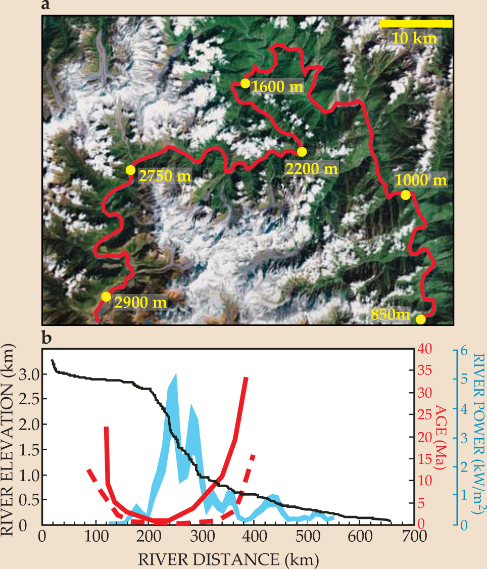
A second example comes from the Namcha Barwa region of eastern Tibet, the edge of an extensive zone of deformation caused by collision of the Indian and Eurasian plates. Here the Yarlung Tsangpo River drops nearly 3 km in elevation as it winds through a small but rugged mountain range, cutting a deep gorge and carrying away large amounts of eroded sediment. Lehigh University geochronologist Peter Zeitler and colleagues have suggested that Namcha Barwa is a crustal aneurysm, where extremely fast rock uplift is fed by deeper flow of hot, ductile rock caught between converging plates.
In their scenario, crustal flow and rock uplift are focused into a narrow zone by the enormous erosive power of the river as it descends through the mountains and carves its deep gorge. Thus thermochronological ages should be lowest where the river is steepest and carries away rock most rapidly. Figure 5 shows that such is indeed the case. The form of the landscape in the Namcha Barwa region may not necessarily change much over time, because erosion keeps pace with the uplift. Observations from other mountain ranges, including those where high erosion is caused by focused precipitation, have motivated a great deal of interest in the nature of feedbacks between processes at the surface and those deep in Earth’s crust and mantle.

Figure 5. Thermochronological age and river slope are related in the Namcha Barwa region of eastern Tibet. (a) The Yarlung Tsangpo River (red) drops rapidly in elevation (values given are in meters above sea level) as it winds through the mountains of Namcha Barwa. (Image obtained from Google Earth, via Peter Zeitler.) (b) Plotted together are elevation (black), mean annual river power (blue), and ages for two thermochronological systems—the biotite K–Ar system (solid red) and the zircon (U–Th)/He system (dashed red). The biotite system has a higher closure temperature than the zircon system and a correspondingly greater depth at which the closure temperature is reached. As a result, ages measured in the biotite system are greater than in the zircon system. For both systems, low ages correspond to high erosion rates and occur in the region of the river’s steepest descent. That result is consistent with a crustal aneurysm model in which broad-scale crustal flow feeds localized rock uplift that is focused by high erosion.
(Adapted from N. J. Finnegan ,
Rates of landscape evolution
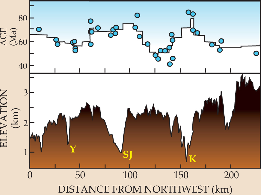
Even in tectonically inactive landscapes, it can be difficult to determine the time scale over which topographic features develop. Some landscapes may change dramatically over short time periods, particularly in response to major climate transitions. But others, including some with dramatic relief, may be little changed for tens or hundreds of millions of years. The imposing and rugged relief of the Sierra Nevada in California has been the focus of debate for decades. The range hosts deep valleys, such as the Kings and San Joaquin canyons, and Mount Whitney—at 4.4 km above sea level, the highest peak in the contiguous US. Some Earth scientists think the Sierra’s dramatic relief has persisted since the time of major plate tectonic convergence in the area, about 60–90 million years ago. Others interpret it as a sign of uplift and incision that occurred relatively recently—perhaps less than 10 million years ago.
A pioneering study from 1998 reached a provocative and still controversial conclusion. Geologist Martha House and coworkers showed that samples collected at about the same elevation along the Sierra Nevada had very different apatite (U–Th)/He ages, depending on their proximity to major valleys such as the Yosemite and San Joaquin canyons. As figure 6 shows, samples near canyons had much higher ages. The simplest explanation for that result is that as samples were exhumed, they passed through Tc at a depth that depended on the overlying topography, as in figure 1. If so, the major range-traversing canyons seen today must have been present in roughly the same positions about 60–80 million years ago, when dinosaurs were walking around in them.

Figure 6. Samples collected near valleys in the Sierra Nevada have higher ages than samples collected at the same elevation but farther from the valleys. The lower panel shows the elevation of the mountains along the line from which the samples were collected. Indicated are the Yosemite (Y), San Joaquin (SJ), and Kings (K) canyons. The upper panel shows the apatite (U–Th)/He ages for the samples (blue circles) along with a running average (stepped curve). The data suggest that samples near major canyons passed through their closure isotherms earlier than samples away from the canyons because of the downward warping of isotherms beneath wide valleys.
(Adapted from M. A. House, B. P. Wernicke, K. A. Farley,
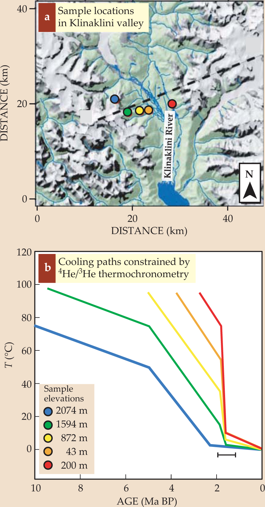
Deeply incised canyons are common in many mountainous areas. Some of the most impressive are the glacial fjords of the Coast Mountains of British Columbia, Canada. In contrast to the ancient Sierran canyons, at least some of them formed relatively recently. Using the method described in figure 3, a team led by one of us (Shuster) analyzed the (U–Th)/He ages of crystals from the region’s Klinaklini valley in combination with intracrystalline 4He concentration distributions. As figure 7 shows, material collected from the bottom of the valley cooled rapidly from about 80 °C to near surface temperature about 1.8 million years ago. Samples collected 2 km higher, from the top of the adjacent ridge, cooled relatively slowly over a period extending from 5 to 10 million years ago. Samples at intermediate elevations display thermal histories that interpolate between those of the end samples. The results of the Shuster study indicate that essentially all the valley’s presently observed relief formed about 1.8 million years ago. Paleoclimate proxies indicate that the same time marks a shift to the 40 000-year cycle for the tilt of Earth’s axis, cooler mean surface temperatures, increased climate variability, and repeated glacial cycles. Apparently, those changes are associated with the onset of rapid glacial erosion and development of high topographic relief in coastal British Columbia.

Figure 7. Samples collected at low altitude in the Klinaklini valley in British Columbia, Canada, cooled more rapidly than those collected higher up. (a) The map shows the present topography of the Klinaklini valley and the locations of five samples analyzed. (b) Model cooling paths corresponding to the color-matched samples in panel a, as constrained by helium-4/helium-3 thermochronological data. Together, the samples suggest an episode of rapid cooling 1.8 ± 0.1 million years ago (indicated by the black bar) associated with roughly 2 km of valley deepening.
(Adapted from D. L. Shuster ,
By constraining the thermal histories of rocks, thermochronology provides a versatile and powerful tool for understanding tectonics and geomorphology. As with any analytical technique, its application must overcome distinctive challenges that can complicate interpretations. For example, ages and daughter product concentration gradients, even together, don’t absolutely constrain a sample’s t–T path, not to mention that the data include experimental uncertainties. Nonetheless, many of the challenges in thermochronology present opportunities to address new types of problems. To give one example, subsurface fluid circulation can complicate the translation of thermal histories into exhumation histories, but under the right circumstances, thermochronological data may reveal much about subsurface fluid flow. Thermochronology is an adaptable technique. Throughout its history, as the subsurface example indicates, it has often been able to turn lemons into lemonade.
References
1. M. H. Dodson,“Closure Temperature in Cooling Geochronological and Petrological Systems”, Contrib. Mineral. Petrol. 40, 259 (1973). https://doi.org/10.1007/BF00373790
2. M. A. House, B. P. Wernicke, K. A. Farley,“Dating Topography of the Sierra Nevada, California, Using Apatite (U–Th)/He Ages,” Nature 396, 66 (1998). https://doi.org/10.1038/23926
3. I. McDougall, T. M. Harrison, Geochronology and Thermochronology by the 40Ar/39Ar Method, 2nd ed., Oxford U. Press, New York (1999).
4. P. K. Zeitler et al.,“Erosion, Himalayan Geodynamics, and the Geomorphology of Metamorphism,” GSA Today 11, 4 (2001). https://doi.org/10.1130/1052-5173(2001)011<0004:EHGATG>2.0.CO;2
5. J. A. Spotila et al.,“Controls on the Erosion and Geomorphic Evolution of the San Bernardino and San Gabriel Mountains, Southern California,” Geol. Soc. Am. Spec. Pap. 365, 205 (2002).
6. P. W. Reiners, T. A. Ehlers, eds., Low-Temperature Thermochronology: Techniques, Interpretations, and Applications, Mineralogical Society of America, Chantilly, VA (2005).
7. D. L. Shuster et al.,“Rapid Glacial Erosion at 1.8 Ma Revealed by 4He/3He Thermochronometry,” Science 310, 1668 (2005). https://doi.org/10.1126/science.1118519
8. J. Braun, P. van der Beek, G. Batt, Quantitative Thermochronology: Numerical Methods for the Interpretation of Thermochronological Data, Cambridge U. Press, New York (2006).https://doi.org/10.1017/CBO9780511616433
9. P. W. Reiners M. T. Brandon,“Using Thermochronology to Understand Orogenic Erosion,” Annu. Rev. Earth Planet. Sci. 34, 419 (2006). https://doi.org/10.1146/annurev.earth.34.031405.125202
10. N. J. Finnegan et al.,“Coupling of Rock Uplift and River Incision in the Namcha Barwa–Gyala Peri Massif, Tibet,” Geol. Soc. Am. Bull. 120, 142 (2008). https://doi.org/10.1130/B26224.1
More about the authors
Peter Reiners is an associate professor of geosciences at the University of Arizona in Tucson. David Shuster is an isotope geochemist at the Berkeley Geochronology Center in Berkeley, California.
Peter W. Reiners, 1 University of Arizona, Tucson, US .
David L. Shuster, 2 Berkeley Geochronology Center, Berkeley, California, US .


