The tangled tale of phase space

Hamiltonian Mechanics is geometry in phase space.

—Vladimir I. Arnold (1978)

Listen to a gathering of scientists in a hallway or a coffee house, and you are certain to hear someone mention phase space. Walk down the science aisle of the local bookstore, and you will surely catch a glimpse of a portrait of a strange attractor, the powerful visual icon of phase space. Though it was used originally to describe specific types of dynamical systems, today “phase space” has become synonymous with the idea of a large parameter set: Whether they are stock prices in economics, the dust motes in Saturn’s rings, or high-energy particles in an accelerator, the degrees of freedom are loosely called the phase space of the respective systems. The concept and its name are embedded in our scientific fluency and cultural literacy. In his popular book Chaos on the history and science of chaos theory, James Gleick calls phase space “one of the most powerful inventions of modern science.” ¹ But who invented it? Who named it? And why?

The origins of both the concept of phase space and its name are historically obscure—which is surprising in view of the central role it plays in practically every aspect of modern physics (figure 1). The historical origins have been further obscured by overly generous attribution. In virtually every textbook on dynamics, classical or statistical, the first reference to phase space is placed firmly in the hands of the French mathematician Joseph Liouville, usually with a citation of the 1838 paper in which he supposedly derived the theorem on the conservation of volume in phase space. ² (The box on page 34 gives a modern derivation.) In fact, in his paper Liouville makes no mention of phase space, let alone dynamical systems. Liouville’s paper is purely mathematical, on the behavior of a class of solutions to a specific kind of differential equation. Though he lived for another 44 years, he was apparently unaware of his work’s application to statistical mechanics by others ³ even within his lifetime. Therefore, Liouville’s famous paper, cited routinely by all the conventional textbooks, and even by noted chroniclers of the history of mathematics, as the origin of phase space, surprisingly is not!

How did we lose track of the discovery of one of our most important modern concepts in physics? If it was not discovered by Liouville, then by whom and when and why? And where did it get its somewhat strange name of “phase” space? Where’s the phase?

The search for the origins of phase space presents two challenges. The first is to identify those people who contributed to the development of the concept of phase space. To do that, we will start back at the time of Liouville to find out what role he really did play in the story and how his contribution found its way into modern textbooks. The second challenge is to discover who gave phase space its fully modern name. To answer that question, we will be led to a now obscure encyclopedia article published in 1911 that had etymological side effects not fully intended by its authors.

Liouville’s theorem

Liouville (1809-82) was perhaps the most renowned French mathematician of the mid-19th century. That era was the golden age of differential calculus and the beginning of differential geometry. Liouville displayed a virtuoso breadth of expertise in topics ranging from number theory and complex analysis to differential geometry and topology. He is known among mathematicians and physicists for several mathematical theorems, most notably the Sturm-Liouville theory of integral equations. The motivation for much of his work came from physical problems in celestial mechanics, but he also drew from electrodynamics and the theory of heat. The properties and solutions of differential equations of many variables were among his main areas of interest, and in that context he was working on the solution of differential equations with constant integrals in the late 1830s.

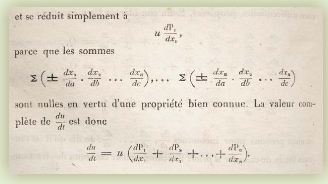
In modern notation, the original formulation of Liouville’s theorem ² (figure 2) states that given a system of n first-order differential equations

$$\frac{d{x}_i}{dt}=p_i\left(t,x_1,x_2,\mathrm{\dots },x_n\right),$$

if a complete set of solutions is

$$x_i=x_i\left(t,a_1,a_2,\mathrm{\dots },a_n\right),$$

where the a_i are arbitrary constants, then the Jacobian determinant

$$u\left(t\right)=\text{det}\left(\frac{\partial x_i}{\partial a_j}\right)$$

satisfies the equation

$$\frac{du}{dt}=\left(\sum _{i=1}^n\frac{\partial P_i}{\partial x_i}\right)u.$$

If the expression in parentheses is zero, then u is a constant. Furthermore, if the arbitrary constants a_i are chosen to be values of x_i at time t = 0, then the system has the solution

$$u\left(t\right)=\text{det}\left(\frac{\partial x_i\left(t\right)}{\partial x_j\left(0\right)}\right)=1$$

because u(0) is clearly equal to 1.

Liouville’s 1838 paper appeared only a few years after William Rowan Hamilton (1805-65) published his dynamics ⁴ in 1834 and 1835, yet Liouville made no reference to his theorem’s application to dynamics.

The connection with mechanics was made in 1842 by the Prussian mathematician Carl Gustav Jacob Jacobi (1804-51), who recognized that the differential equations that Liouville had studied could describe mechanical systems ⁵ (figure 3). In Hamilton’s dynamics, position coordinates x_i and momentum coordinates p_i evolve according to the Hamiltonian function H:

$$\frac{d{x}_i}{dt}=\frac{\partial H}{\partial p_i},\hspace{0.17em}\frac{d{p}_i}{dt}=-\frac{\partial H}{\partial x_i}\cdot$$

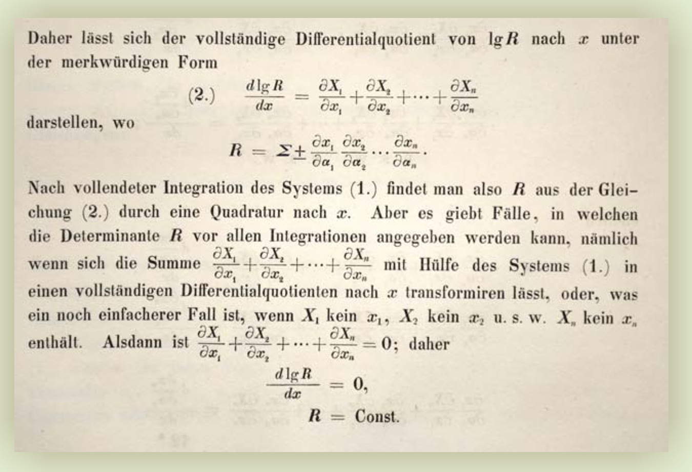
To apply Liouville’s theorem, Jacobi made the assignments (again in modern notation)

$$\begin{array}{c}{x}_{i=1:n}=x_{i=1:n},\hspace{0.17em}{x}_{i=n+1:2n}=p_{i=1:n};\\ P_{i=1:n}=\frac{\partial H}{\partial p_i}{{|}_{i=1:n},P_{i=n+1:2n}=-\frac{\partial H}{\partial x_i}|}_{i=1:n}\end{array}$$.

Therefore,

$$\sum _{i=1}^{2n}\frac{\partial P_i}{\partial x_i}=\sum _{i=1}^n\frac{{\partial }^{2}H}{\partial x_i\partial p_i}-\sum _{i=1}^n\frac{{\partial }^{2}H}{\partial p_i\partial x_i}=0,$$

and, according to Liouville’s observation, the Jacobian determinant u is constant.

Explicitly referencing Liouville’s 1838 paper in the 1866 publication of his lectures of 1842-43, Jacobi was the first to put Liouville’s mathematical theorem into a mechanical context. What Jacobi did not do, and indeed could not do in his time, was to represent mechanical systems within a generalized space. In the early 1840s, there was no concept of space beyond our physical three dimensions. That was slightly before Arthur Cayley, Hermann Grassmann, and Bernhard Riemann presented their new notions of multidimensional manifolds. For Jacobi, there was no “space,” only products of differentials of many variables. And there certainly were no trajectories through the phase space, only the physical trajectories of individual particles through real space. Therefore, Jacobi may be the originator of the analytical treatment of dynamical systems of many variables, but he cannot be designated as the originator or namer of phase space. The time was not right. First, the concept of multidimensional spaces had to enter the psyche of 19th-century scientists.

Fermat’s “etc.”

About the time that Liouville was studying differential equations of many variables, German and British mathematicians were taking the first steps toward expanding the notion of space. The invention of spaces of dimensions higher than three was gradual, not occurring in a single “aha!” moment but developing over many years with some, like the German geometer Julius Plücker, circling it in the early 1840s but failing to hit it quite on the nose.

Equations of multiple variables had been around for a long time. As far back as the mid-17th century, Pierre de Fermat noted, “In the first problems we seek a unique point, in the latter a curve. But if the proposed problem involves three unknowns, one has to find, to satisfy the equation, not only a point or a curve, but an entire surface. In this way surface loci arise, etc.” Fermat’s “etc.” may be the first hint of solutions existing in higher dimensions. Those ideas were developed further in the 18th century by Immanuel Kant, Jean d’Alembert, and Leonhard Euler. Today it is natural for us to assign each variable its own axis in a generalized multidimensional space. But in the 1700s it was not natural. Variables were algebraic entities, not coordinate axes. And while the solutions to equations of multiple variables could lead to loci of points with multiple indices, there was no formal thought that they represented geometric objects in higher dimensions. Amazingly, the surface areas and volumes of spheres in four dimensions (and higher) had been derived by Jacobi as early as 1834, but to him they were simply integrals over products of differentials.

All that would change rather suddenly in the 1840s as Plücker in Germany and Cayley and James Joseph Sylvester in the UK parameterized projective geometry and found extensions beyond the ordinary three dimensions of our tangible world. Cayley, in his 1843 paper titled “Chapters in the Analytical Geometry of (n) Dimensions,” was the first to take the bold step of referring to a geometry of more than three dimensions. After that, the stage was set for the “invention” of multiple dimensions when Grassmann developed the concept of an n-dimensional vector space in 1844. The culmination of the multidimensional trend in analytic geometry came with Riemann’s lecture on the foundations of geometry, delivered at the University of Göttingen in 1854, in which he systematized concepts of curved spaces that were later to be so important for general relativity.

Riemann’s work remained obscure until its publication in 1868, after which the geometric properties of multidimensional manifolds were developed rapidly by many others, most notably by Enrico Betti, Felix Klein, and Camille Jordan in the 1870s. That was the same decade that a brilliant young Austrian physicist, Ludwig Boltzmann, laid the foundations of the new field of statistical mechanics.

Boltzmann’s phase

Boltzmann (1844-1906) received his PhD under Joseph Stefan at the University of Vienna in 1866 with a dissertation on the kinetic theory of gases. In the derivation of dynamical probability distributions, Boltzmann required the use of what we now know as conservation of volume in phase space. Initially unaware of Jacobi’s original work or of the connection with Liouville, he derived that principle using an approximation that he published in early 1871. ⁶ However, in his very next paper, published later that same year, ⁷ Boltzmann made explicit use of Jacobi’s results to derive the conservation theorem

$$d{x}_1\left(t\right)d{x}_2\left(t\right)\mathrm{\dots }d{x}_{2n}\left(t\right)=\left|\frac{\partial x_i\left(t\right)}{\partial x_j\left(0\right)}\right|d{x}_1\left(0\right)d{x}_2\left(0\right)\mathrm{\dots }d{x}_{2n}\left(0\right),$$

where

Despite Jacobi’s reference to Liouville’s theorem in his 1866 Vorlesungen über Dynamik (Lectures on Dynamics) , Boltzmann made no mention of Liouville at this time. His seminal 1871 papers contain no language of “phase” or “space,” although the conservation of what would later be called phasespace volume for a conservative dynamical system appears in its mathematically modern form.

The second 1871 paper is where Boltzmann first makes the analogy ^{7 , 8} between physical trajectories of particles in two-dimensional space and what are known as Lissajous figures (although he does not refer to Jules Antoine Lissajous). Lissajous figures, also sometimes called Bowditch-Lissajous figures after the scientist and navigator Nathaniel Bowditch, are two-dimensional patterns that arise when two harmonic time series are plotted against each other—as best experienced in physics labs using an oscilloscope and two function generators. When the two harmonic frequencies are rational fractions, periodic patterns occur. But when the frequency ratio is irrational, the system trajectory visits all points on the plane bounded by the signal amplitude. That is Boltzmann’s first description of what would later become his ergodic hypothesis, ⁹ which states that a dynamical system samples all parts of its dynamical space.

In Lissajous figures, the relative phase between the harmonic signals plays an important role in determining the pattern, and the instantaneous point on the figure defines the instantaneous relative phase of the two signals. For that reason, the point on the figure is referred to as the phase point. In 1872 Boltzmann used the term “phase” for the first time in a paper on the further studies of the equipartition theory of gas molecules. ¹⁰ “Phase” is not applied in that first case to the system trajectory of the gas, which would have been the direct analogy with Lissajous figures. However, because of the complicated motions of the atoms in molecules, Boltzmann made the distinction between kind of motion (Bewegungsart, such as translational and rotational motion, which contribute to the total energy) and the phase of the motion (Bewegungsphase, such as the changing coordinate and momentum values of the motion). That is the defining moment for the word “phase” in phase space.

Examining Boltzmann’s work in 1879, James Clerk Maxwell (1831-79) adopted Boltzmann’s expression of phase to describe the state of a system:

We have hitherto, in speaking of a phase of the motion of the system, supposed it to be defined by the values of the n co-ordinates and the n momenta. We shall call the phase so defined the phase (pq). ¹¹

In his paper, Maxwell rederived the conservation theorem, explicitly using Hamilton’s equations to show that the Jacobian determinant was unity. Maxwell’s rederivation was consistent with Liouville’s 1838 theorem but did not explicitly use it.

Boltzmann, for his part, did not use the term “phase” after his 1872 paper until the publication of his Vorlesungen über Gastheorie (Lectures on Gas Theory) in 1896. Also missing from Boltzmann’s stream of papers through the 1870s and 1880s is any geometric language. Despite the multidimensional volume integrals that appear frequently in his papers, the volume elements are merely products of the differentials of multiple variables, and the integrals themselves are never described as multidimensional volume integrals. His lack of geometric language is interesting in view of the fact that multidimensional spaces were becoming more broadly accepted at the time.

That all changed with the appearance of Boltzmann’s Lectures in 1896, in which he took a more direct attitude toward geometry and referred to n-fold integrals over n-fold regions. Boltzmann took a tantalizing step in the direction of describing a single trajectory of the system through its dynamical space:

When one wishes to discuss any curve whose equation contains an arbitrary parameter, it is customary to consider simultaneously all the curves obtained by giving this parameter all its possible values. We are now dealing with a mechanical system (characterized by given equations of motion) whose motion depends on the values of the 2µ parameters P, Q. ¹²

That view of a dynamical system as a single trajectory is made by analogy to a curve rather than made explicitly. Boltzmann still does not seem able to take that final step of speaking of a single trajectory through a multidimensional space. All the mathematics is in place, and he makes the analogies and uses the geometric language of n-fold regions, but he implies the trajectory rather than stating it explicitly. That inability is clearly related to the fact that he never uses the word “space,” and thus does not take the last step to call it “phase space.”

One of the questions posed at the beginning of this article can be answered here. Why does Liouville get the credit when it was Jacobi and Boltzmann who invented phase space and discovered conserved volumes in it? The answer is that Boltzmann himself gives Liouville the credit in his Lectures. Although Boltzmann had known, at the time of his early papers, of Jacobi’s reference to Liouville’s theorem, it was only later in his Lectures of 1896 that Boltzmann first placed Liouville’s name on the conservation theorem in a way that stuck. ³ Had it not been for Jacobi’s reference to Liouville in his Lectures , Boltzmann likely never would have known of Liouville’s paper. In turn, had Boltzmann not given the credit to Liouville, then the conservation of phase-space volume could very reasonably have been called Boltzmann’s theorem. Ironically, by naming it “Liouville’s Theorem” Boltzmann obscured his own role in the discovery and use of phase space.

If Boltzmann had used the language of system trajectories in his original papers from 1871, it would have been astounding. He would have been far ahead of his time in the abstract representation of the complicated motions of multiple particles in a single three-dimensional space as a single point moving in a multidimensional space. On the other hand, only a few years after Boltzmann’s Lectures , the American physicist J. Willard Gibbs (1839-1903), writing in his Elementary Principles in Statistical Mechanics in 1902, did express this view:

If we regard a phase as represented by a point in space of 2n dimensions, the changes which take place in the course of time in our ensemble of systems will be represented by a current in such space. ¹³

Here we see, for the first time, the explicit reference to the trajectory of the phase point in a high-dimensional space. However, even in Gibbs’s Elementary Principles there remain hesitations. Although he rederived the conservation of phasespace volume, he did not use the word “volume” but instead used Grassmann’s term, “extension.” Even more telling is that the only place Gibbs used the word “space” is in a footnote, as if the notion of a trajectory in a high-dimensional space was an aside or an analogy, literally a footnote, rather than a fundamental principle. So even Gibbs was not immune to the prejudices about space at the turn of the century. Although he was a great inventor of terminology, giving us “statistical mechanics” and “ensemble” and establishing the modern nomenclature of vector analysis, he did not invent the phrase “phase space.” Nor did he invent the concept of the system trajectory. That had come from the pioneering work of Henri Poincaré.

Poincaré’s tangle

Poincaré’s part in the story of phase space began with the announcement in 1885 of a mathematical prize to be offered in honor of the 60th birthday of King Oscar II of Sweden. The idea of the prize had been suggested to the king by Swedish mathematician Gösta Mittag-Leffler. The topic of the prize was to be the problem of finding a general solution to the stability of the solar system. The announcement stated the problem: “Given a system of arbitrarily many mass points that attract each other according to Newton’s law, under the assumption that no two points ever collide, try to find a representation of the coordinates of each point as a series in a variable that is some known function of time and for all of whose values the series converges uniformly.” The simplest n-body problem was the three-body problem that had defied the efforts of the world’s most renowned mathematicians, including Isaac Newton and Euler.

Poincaré (1854-1912) was attracted by the similarity between the stated goal of the prize and a topic on which he had already done much preliminary work. His work in the 1880s had focused on the global behavior of dynamical curves that approached steady-state solutions that were either points (called fixed points) or closed curves (called limit cycles).

Poincaré decided to formulate the prize problem in the very simple terms of two gravitating bodies to which a third is added whose mass is so small as to make negligible perturbations on the motions of the original two. Poincaré thought he was able to prove that the motion of the third body was technically stable, returning arbitrarily closely to its original position if given sufficient time.

Even though Poincaré did not solve the original problem, his contributions were deemed the most worthy of the entrants, and he was awarded the prize on 21 January 1889. As part of the prize process, he wrote up his essay for publication in Acta Mathematica. The paper was already through proofs and initial printing late in 1889 when, upon checking one of his most important conclusions, he discovered an error. He had originally intended to show that if the motion of the small body were perturbed slightly, it would remain arbitrarily close to the original motion. But upon studying his results further (after attempting to respond to a reviewer’s comments on his manuscript), he discovered that was not true. In fact, he found that arbitrarily small perturbations could lead to arbitrarily large changes in the motion. If one viewed Earth as the small body, it raised potentially important questions about Earth’s future in the solar system.

By then Poincaré had to scramble. He informed the committee of the error, worked feverishly from December 1889 to January 1890 to correct the manuscript, and then paid for the reprinting of the journal volumes out of his own pocket. That the published paper was not the original submission to the prize committee was apparently not widely known until the 1990s. ¹⁴

In the course of correcting his mistake, Poincaré took a geometric approach in which he visualized the behavior around a special feature of the motion called a homoclinic fixed point—a saddle point where stable and unstable trajectories intersect in phase space. As he studied the solutions, he discovered that the trajectories would cross an infinite number of times. It was that “tangle” (figure 4) that was generating the arbitrarily large response to small changes in initial conditions that he had discovered. He was amazed by his own findings:

If one seeks to visualize the pattern formed by these two curves and their infinite number of intersections … these intersections form a kind of lattice-work, a weave, a chain-link network of infinitely fine mesh; each of the two curves can never cross itself, but it must fold back on itself in a very complicated way so as to recross all the chain-links an infinite number of times … One will be struck by the complexity of this figure, which I am not even attempting to draw. Nothing can give us a better idea of the intricacy of the three-body problem, and of all the problems of dynamics in general. ¹⁵

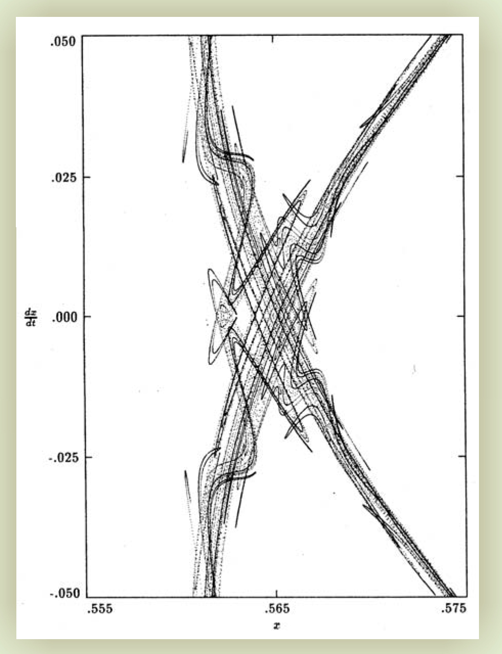
It was clear to him that he had discovered a fundamentally new aspect of dynamical motion. That was the original discovery of what is today known as sensitivity to initial conditions, which is at the heart of chaos theory.

Poincaré completed his studies of dynamic motion and published his results in three volumes under the title New Methods of Celestial Mechanics. ¹⁵ He carried out much of the work in phase space, introducing new tools and geometric approaches that have become workhorses of modern dynamics. Among his contributions are Poincaré sections, which plot where trajectories intersect a specified section of phase space (see figure 1), and fixed-point classifications that categorize various types of equilibrium behavior. The third volume of New Methods contained the material introducing chaotic motion arising from the homoclinic tangle. Along the way, Poincaré derived the theorem on the conservation of phase space, which he called an integral invariant; he was unaware of its derivation by Boltzmann, who in turn had at first been unaware of Jacobi’s original derivation.

Ehrenfests’ legacy

The “space” aversion at the end of the 19th century quickly evaporated in the first decade of the 20th, especially with the advent of relativity and the growing conception of four-dimensional spacetime, in which time takes on some of the properties of a fourth spatial dimension, a viewpoint developed by Hermann Minkowski in 1907. Boltzmann by that time was dead (by his own hand), but one of his students, Paul Ehrenfest (1880-1933), was asked by Felix Klein to write a review of Boltzmann’s work for the Encyclopedia of Mathematical Sciences. Ehrenfest, with his physicist wife, Tatyana, published the encyclopedia article in 1911. ¹⁶ They approached the subject systematically, seeking to make precise definitions. That care was partly in response to the controversies that had raged during the later part of Boltzmann’s life over proofs or disproofs of the ergodic nature of gas systems. The Ehrenfests took great pains to define a rigorous name for the multidimensional dynamical space—and invented the term “ Γ-space” in that space the instantaneous state of the system was the Γ-point.

There are ironies here. By the time of the encyclopedia article, the stigma of using the expression “space” for multiple dimensions had disappeared, and the Ehrenfests were very comfortable using the term to define Boltzmann’s n dimensions. But possibly because of its obscurity, they dispensed with the term “phase” that Boltzmann so liked. Yet at the beginning of the encyclopedia article, to set the context for their newly coined term of Γ-space, they needed to refer back to Boltzmann’s usage of “phase.” To do so, they briefly mention Phasenraum (phase space) in the article and then immediately dispense with it, never to use it again. That throw-away phrase is apparently the first use of the expression “phase space” in print.

Encyclopedia articles in the Ehrenfests’ day were widely read, somewhat like Reviews of Modern Physics today, and the Ehrenfests’ article was no exception. And here is the main irony: What stuck in readers’ minds was the toss-away phrase “phase space,” while virtually everyone ignored the Γ-space invention.

Within two years of the Ehrenfests’ article, two papers—by Artur Rosenthal (1887-1959) and by Michel Plancherel (1885-1967), both on ergodic theory—in the same 1913 issue of Annalen der Physik used the expression “phase space” for the first time in journal publications. ¹⁷ The usage stuck, first appearing in a journal paper title in 1918 ¹⁸ and becoming increasingly common after that. As a side note, Rosenthal later became a professor of mathematics at Purdue University. My close colleague Anant Ramdas at Purdue remembers him, so we have still today a living connection—in the “six degrees of separation” sense—from Rosenthal to the Ehrenfests to Boltzmann to Jacobi to Liouville.

References

1. J. Gleick, Chaos: Making a New Science, Viking, New York (1987).
2. J. Liouville, J. Math. Pures Appl. 3, 342 (1838).
3. J. Lu¨tzen, Joseph Liouville, 1809–1882: Master of Pure and Applied Mathematics, Springer, New York (1990).
4. W. R. Hamilton, Philos. Trans. R. Soc. London 124, 247 (1834); https://doi.org/10.1098/rstl.1834.0017
125, 95 (1835). https://doi.org/10.1098/rstl.1835.00095. C. G.J. Jacobi, Vorlesungen u¨ber Dynamik, Georg Reimer, Berlin (1866).
6. L. Boltzmann, Wien. Ber. 63, 397 (1871).
7. L. Boltzmann, Wien. Ber. 63, 679 (1871).
8. S. Brush, The Kinetic Theory of Gases: An Anthology of Classic Papers with Historical Commentary, Imperial College Press, London (2003).
9. L. Boltzmann, Sitzungsber. Akad. Wiss. Wien, Math.-Naturwiss. Kl. 90, 231 (1884).
10. L. Boltzmann, Wien. Ber. 66, 275 (1872).
11. J. C. Maxwell, Trans. Cambridge Philos. Soc. 12, 547 (1879).
12. L. Boltzmann, Vorlesungen u¨ber Gastheorie, J. A. Barth, Leipzig, Germany (1896–98)
;
Lectures on Gas Theory, S. G. Brush, trans., Dover, New York (1995).13. J. W. Gibbs, Elementary Principles in Statistical Mechanics, Scribner, New York (1902).
14. J. Barrow-Green, Poincare´ and the Three Body Problem, American Mathematical Society, Providence, RI (1997).
15. H. Poincare´, New Methods of Celestial Mechanics, D. L. Goroff, ed., American Institute of Physics, New York (1993).
Reprinted from Les me´thodes nouvelles de la me´canique ce´leste, Gauthier-Villars, Paris (1892–99).16. P. Ehrenfest, T. Ehrenfest, in Encyklopa¨die der mathematischen Wissenschaften, vol. 4, part 32, B. G. Teubner, Liepzig, Germany (1911).
17. A. Rosenthal, Ann. Phys. (Leipzig) 42, 796 (1913);
M. Plancherel, Ann. Phys. (Leipzig) 42, 1061 (1913).18. P. S. Epstein, Abh. Preuss. Akad. Wiss. 23, 435 (1918).
More about the authors
David Nolte is a professor of physics at Purdue University in West Lafayette, Indiana.
David D. Nolte, Purdue University, West Lafayette, Indiana, US .