The power of imaging with phase, not power
DOI: 10.1063/PT.3.3553

’Tis such a long way to the star
Rising above our shore–
It took its light to come this far
Thousands of years and more.
It may have long died on its way
Into the distant blue,
And only now appears its ray
To shine for us as true.
—Mihai Eminescu. From “Unto the Star,” 1886. English translation by Adrian G. Sahlean
In the 17th century, the microscope and telescope played decisive roles in the scientific revolution. Stars and planets, though enormous, are so distant that they appear as pinpricks in the sky. The telescope made them appear nearer, so the viewer could now discern that Saturn had rings, Jupiter had moons, and the Milky Way was composed of a myriad of stars. The microscope accomplished the opposite of sorts: It magnified microorganisms, human cells, and other earthly but minuscule objects and made them visible to the eye.
However, early microscopists quickly discovered how challenging it is to image cells and other transparent objects. Because all detectors, including the human retina, are sensitive to light power and because most cells do not absorb or scatter light significantly, early images of them lacked contrast.
In the late 19th and early 20th centuries, biologists developed new methods to artificially generate contrast by chemically binding stains and fluorophores to biological structures of interest. To this day microscopic investigation of stained biopsies remains the gold standard in pathology, and fluorescence microscopy has become the preferred imaging tool in cell biology.
Exogenous contrast mechanisms enable investigators to label particular structures of interest. However, adding foreign chemicals to a living cell is bound to affect its function. Fluorescence excitation light, often in the UV, has proven toxic to cells. Furthermore, fluorescence molecules can suffer photobleaching: irreversible chemical changes that quench the fluorescence and limit the interval of continuous imaging to only a few minutes.
Phase contrast microscopy was developed in the 1930s as a means to generate contrast without exogenous contrast agents. It exploits the phase change that occurs when light interacts with a transparent object. Although useful for nondestructively visualizing internal structures of cells and tissues, phase contrast microscopes do not quantify the amount of phase delay induced by the imaged object.
Quantitative phase imaging (QPI) specifically focuses on extracting the optical path-length maps associated with specimens. Unlike traditional microscopes that use one beam of light for imaging, QPI instruments detect the superposition, or interference, of two beams: an object beam that interacts with the sample and a reference beam that does not. In effect, QPI combines the principles of interferometry, microscopy, and holography.
Rapid progress in instrument development over the past decade has led to the commercialization of several flavors of QPI devices. Naturally, research focus has shifted from instrument development to biomedical applications. In this article I place QPI in its historical context, describe the main experimental approaches, and present some of the important applications.
Interferometry
Perhaps no other experimental method has transformed science at a deeper, more fundamental level than light interferometry. Thomas Young’s 1803 experiment,
1
illustrated in figure

Figure 1. Highlights in interferometry. (a) Thomas Young’s 1803 two-slit interference experiment laid the foundations for the wave theory of light. (Adapted from ref.
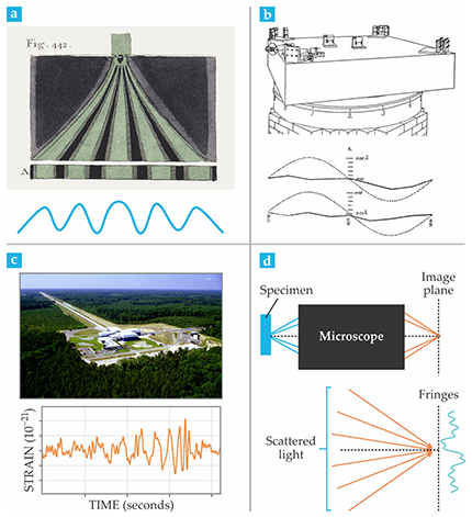
Toward the end of the 19th century, Albert Michelson perfected a type of interferometer that was quite different from Young’s. In addition to producing spatial fringes, Michelson’s interferometer generated a temporal interferogram: fringes with respect to the time delay between the two interfering waves. Michelson used his interferometer to define the meter in multiples of cadmium-light wavelengths. As a result, in 1907 he became the first American to receive the Nobel Prize in Physics.
Yet, it was the Michelson–Morley experiment
2
that became even more famous. In 1887 Michelson and Edward Morley set out to interferometrically measure the relative motion between Earth and the presumed light-bearing medium, the luminiferous ether. Their failure to detect such motion with their precision apparatus (figure
A similar interferometric geometry was used recently to confirm the existence of gravitational waves predicted by Einstein’s general relativity theory.
3
Although the twin interferometers of the Laser Interferometer Gravitational-Wave Observatory (figure
Microscopy
Interference was understood as a crucial ingredient in image formation as early as 1873, when Ernst Abbe published his breakthrough theory of coherent image formation.
4
To succinctly sum up Abbe’s theory, “The microscope image is the interference effect of a diffraction phenomenon.”
5
In that description, as illustrated schematically in figure
Because a sinusoidal fringe produced by two interfering waves has a period dictated by the wavelength of light and the angle between them, the smallest resolvable feature in the image is related to the angular coverage, or numerical aperture, of the imaging system. Conventional far-field imaging results in a resolution of, at best, half the wavelength of light.
Abbe’s insight into image formation transformed our understanding not only of the microscope’s resolution but also of the contrast it generates when imaging transparent specimens, such as live, unlabeled cells. In the 1930s Frits Zernike reasoned that if the image is just a complicated interferogram, increasing its contrast amounts to increasing the contrast of the fringes formed at the image plane. 5 He treated the image as the result of interference between unscattered incident light and scattered light. He realized that when imaging a highly transparent structure, the scattered field is much weaker than the incident field, and as a result, the two interfere with low contrast.
Furthermore, the intensity at each point in the image depends on the cosine of the phase shift, which describes the interference term. For small phase shifts, the first derivative of the cosine is nearly zero, so the modulation in the intensity is small and the contrast is low. Zernike’s solution was to simply impose an additional quarter-wavelength shift between the incident and scattered fields. He did so by inserting a thin metallic filter that he called a phase strip at the position in the back focal plane of the microscope objective where the incident light converges to form an image of the light source. The resulting interference then varies as a sine function, which is approximately linear at the origin; the intensity image therefore exhibits high contrast.
In addition, if the phase strip exhibits significant absorption, as is the case with metals, it also balances the power of the two beams and further boosts the contrast. Suddenly, internal structures of live, unlabeled cells become visible. For his phase contrast microscope, Zernike received the 1953 Nobel Prize in Physics.
Still, the phase contrast image is an intensity map, albeit one that depends on phase in a nontrivial manner. That is why phase contrast microscopy has been used largely as a visualization technique rather than as a method to infer quantitative data.
Holography
By capturing the phase of a field with respect to a reference, one can reconstruct the complex image field without distortion. That is the principle of holography, first demonstrated by Dennis Gabor in the 1940s.
An electrical engineer by training, Gabor introduced the use of complex analytic signals to describe the temporal behavior of electromagnetic waves used in communication. 6 The complex analytic signal, derived by discarding the negative frequency components of the original signal’s spectrum, facilitates many computations involving real-valued electromagnetic fields. In essence, one takes the Fourier transform of the original signal, throws away the negative frequency components, and then performs an inverse Fourier transformation. In that formalism, the phase is well defined as the argument of the complex analytic signal.
Gabor invented a method to create images with complex fields as a means to transmit information over parallel channels. His “new microscopic principle” 7 enabled one to record in a hologram not just the amplitude of the light field but also its phase. Although Gabor originally proposed holography as a method for aberration correction of electron micrographs, optical holography took on a life of its own, with applications spanning from entertainment to secure encoding and data storage. In 1971 Gabor, too, received the Nobel Prize in Physics.
The right combination
Quantitative phase imaging takes the principle of holography a step further and extracts the phase of the field separately from its amplitude. That decoupling is accomplished via interferometry. Figure

Figure 2. Two main configurations for quantitative phase imaging (QPI). (a) In phase-shifting QPI, the reference field propagates along the same axis as the object field. The phase of the reference field is successively shifted by π/2 to produce four images, which are combined to extract the phase shift induced by the specimen. (b) Off-axis QPI tilts the propagation axis of the reference field to produce an interference pattern so that the phase shift due to the specimen is obtained from a single image.
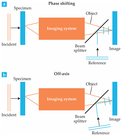
In the phase-shifting approach (figure
In the off-axis approach (figure
However, the speed advantage occurs at the expense of the so-called space–bandwidth product: Compared with phase-shifting methods, there is either some loss of image resolution (spatial bandwidth) or reduced field of view (space). The reduction occurs because the ultimate spatial sampling of the image is no longer the camera pixel but the period of the interferogram.
Phase-shifting methods maximize the space–bandwidth product but reduce the time–bandwidth product—that is, the product of the duration of the imaging (time) and the temporal resolution (temporal bandwidth). Thus phase-shifting and off-axis methods are complementary and their relative suitability depends on the particular application at hand.
The performance of a QPI method is evaluated in terms of many factors. The most important are spatial resolution, temporal resolution, spatial sensitivity, and temporal sensitivity. 8 Spatial resolution establishes the finest details in the transverse (xy) plane of the specimen that the method can render. Ideally, the spatial resolution approaches its best diffraction-limited value. Temporal resolution is given by the maximum acquisition rate that the instrument provides, and it dictates the fastest dynamic phenomenon that can be studied.
Spatial sensitivity describes the smallest phase change detectable across the xy field of view at an instant of time. High sensitivity is particularly important when imaging extremely thin specimens. Spatial noise is intrinsically affected by the coherence properties of the illumination. For example, laser illumination generates speckle patterns, which result in a noisy background, and thus lowers spatial sensitivity. White-light illumination, on the other hand, averages out the speckles and generates a more uniform background and low spatial noise.
Temporal sensitivity establishes the smallest detectable phase change along the time axis at a fixed point in space. It is related to the stability of the interferometer and is crucial when studying subtle dynamic phenomena that result in small displacements. The most effective way to minimize temporal noise is to design an interferometer in which the two interfering waves traverse a nearly identical physical path. Such common-path interferometers are known to be intrinsically stable.
Applications
The ability to image unlabeled specimens makes QPI ideal for imaging live cells in culture. In particular, red blood cells have been investigated heavily by QPI. Because red blood cells lack nuclei and other internal structures, the phase change depends mostly on the concentration of hemoglobin and the cell thickness. The QPI information can thus be converted easily into topography, as shown in figure

Figure 3. Phase to morphology—phase to mass. (a) The phase shift induced by a red blood cell, which lacks a nucleus, depends on the cell’s thickness. Quantitative phase imaging (QPI), therefore, probes cellular topography. (Adapted from G. Popescu et al., J. Biomed. Opt. 10, 060503, 2005, doi:10.1117/1.2149847 .) (b) For cells that are structurally more complex, the phase image can be turned into a map of the density of dry matter— everything in the cell that is not water. (Adapted from G. Popescu et al., Lab Chip 14, 646, 2014, doi:10.1039/C3LC51033F .) (c) Fourier transform light scattering (FTLS) numerically propagates the information in a QPI image—such as the one here of cultured brain cells—to the momentum, or scattering angle, domain. (d) The angle dependence of scattered intensity in region d from panel c identifies the occupants as protein-filled cell protusions called filopodia. The upper inset shows the phase image of the region at higher magnification. The lower inset is the spatial power spectrum. (e–g) Dispersion-relation phase spectroscopy extends FTLS to dynamic processes—namely, how temporal correlations in the dry-mass density decay as a function of momentum transfer q. Data in each panel are from the correspondingly labeled region in panel c. A linear decay rate Γ (blue curve, measurement; orange curve, fit) indicates active transport of vesicles and organelles; a quadratic Γ indicates passive diffusion.
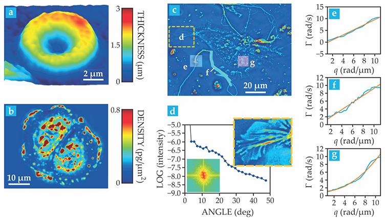
Quantitative phase imaging also has valuable applicability to cells that do contain nuclei and organelles. One of the most useful features of QPI is that the phase image of a cell can be converted into a map of the dry-mass density in the cell (see figure
The procedure, first introduced by Robert Barer in the 1950s in the context of phase contrast microscopy, follows from the fact that the phase shift through a cell immersed in aqueous solution is proportional to the density of dry matter—mainly proteins and lipids. 9 The phase-to-dry-mass-density ratio, it turns out, is relatively constant no matter the protein type that produces the phase shift. That remarkable phase-to-mass equivalence means that QPI can “weigh” cells without contact and track their weight over virtually arbitrary time scales. 10 Understanding cell growth and how it is influenced by environmental factors and disease remains a grand challenge in biology. 11
Quantitative phase images can be used to numerically represent the optical field in the spatial frequency, or momentum, domain. The approach, known as Fourier transform light scattering (FTLS), 12 is analogous to Fourier transform IR spectroscopy, in which a broadband absorption or emission signal is processed through an interferometer in the time domain and then Fourier transformed to yield spectroscopic information.
Analogously, FTLS quantifies the phase shift and amplitude of broadband light scattered by a sample via interferometry. The measured data may be expressed as a complex analytic signal in the spatial domain, and the Fourier transform of that signal conveniently reveals the distribution of scattering angles—or, equivalently, momentum transfer values—and the correlations between the positions of individual scatterers in the sample.
When studying optically thin objects such as cells, FTLS has distinct advantages over traditional angle-resolved measurements in terms of sensitivity because it is performed in the spatial domain. At each point in the image field, the signal is the result of field superposition, or interference, from all available angles. That results in a much higher signal compared with the case in which the power scattered at each angle is measured separately. As shown in figures
Over the past decade, researchers have developed stable QPI systems that are capable of measuring dynamic phenomena in the living cell. The time scales of interest vary over several orders of magnitude: milliseconds to seconds for membrane fluctuations, seconds to minutes for intracellular mass transport, and hours to days for cell growth.
Using the phase-to-mass equivalence discussed previously, QPI has been employed to study the physics of intracellular transport. By measuring a series of phase images at set time intervals, one can track the motion of dry mass, mainly vesicles and organelles, inside a cell. An implementation of FTLS called dispersion-relation phase spectroscopy (DPS) decomposes the data in the spatiotemporal frequency domain.
The correlation between the dry-mass density at a given time and at some later time, called the temporal autocorrelation, decays in time. Experiments have shown that the decay rate has a term that is linear in momentum transfer and one that is quadratic. 13 The linear term describes deterministic, active motion caused by molecular motors, whereas the quadratic term reflects random, passive, diffusive transport.
In neurons, for example, it was found that transport of vesicles along neural filaments (axons and dendrites) is largely deterministic (figures
Red blood cell membrane fluctuations have been studied for decades using interferometric techniques. With the capabilities of the new QPI instruments, the displacements were measured with nanoscale sensitivity, and those data were used to determine the elastic properties of the membrane in both healthy and diseased states. Membrane fluctuations were found to have both deterministic and diffusive components. 14
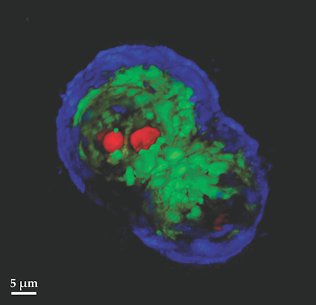
The equivalence between the phase and scattering information can be generalized further to study three-dimensional objects. It has been shown that by acquiring a stack of 2D quantitative phase images along a third axis—which may be angle,
15
the z-axis,
16
or optical frequency
17
—the scattering inverse problem can be solved uniquely and the scattering potential of the object obtained uniquely (figure

Figure 4. Label-free tomography of a colon cancer cell. The false color rendering (red, nucleoli; green, nuclei; purple, membrane) was obtained by combining 140 two-dimensional slices imaged by spatial light interference microscopy. (Adapted from ref.
To the clinic
The label-free and quantitative information extracted from specimens by QPI represents an important opening for hematopathology. Traditional pathology relies on tissue staining and inspection by a trained pathologist. Although the procedure remains the gold standard for now, it is subject to well-documented observer bias and low throughput.
The QPI image of an unstained tissue slice displays the nanoarchitecture of the tissue. Subtle changes in morphology due to the onset of cancer can be easily observed. Figure

Figure 5. Unlabeled prostate core biopsy imaged by quantitative phase imaging (QPI), compared with those traditionally imaged after staining with H&E (hematoxylin and eosin, the most common stain in histopathology). Both images reveal a lack of glandular structure—a hallmark of cancer. Unlike traditional pathology, which relies on pathologists to inspect and evaluate each image, analysis of QPI data can be automated and is not susceptible to observer bias.
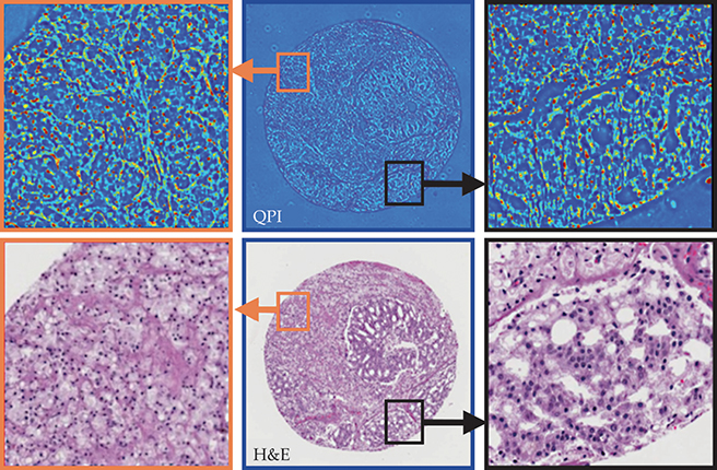
The QPI method used here is spatial light interference microscopy, in which a system comprised of lenses and a phase modulator is added onto a traditional phase contrast microscope. The add-on module spatially separates the scattered and incident light, and then recombines them after modulating the phase of the incident light to produce an interferogram. The QPI data depend on neither staining strength nor color correction. As a result, images can be compared quantitatively across instruments and laboratory locations and thus are suitable for automated analysis.

In the future, large QPI databases could be used to train advanced machine learning algorithms that can identify abnormalities in blood samples. Blood smears could be effectively studied by QPI, and with additional efforts on classifying white blood cells, one could produce a complete blood count from a single finger prick. Blood testing could potentially become a do-it-yourself procedure, similar to glucose testing today. Importantly, such QPI-based blood testing could be performed in the field using portable devices because it would not require infrastructure for processing the sample.
I gratefully acknowledge the scientific contributions of members of the quantitative light imaging lab and the fast growing quantitative phase imaging community and support from NSF (CBET-0939511 STC, DBI 14-50962 EAGER, and IIP-1353368).
References
1. T. Young, A Course of Lectures on Natural Philosophy and the Mechanical Arts, vol. 1 (1807).
2. A. A. Michelson, E. W. Morley, Am. J. Sci. 34, 333 (1887).
3. B. P. Abbott et al. (LIGO collaboration and Virgo collaboration), Phys. Rev. Lett. 116, 061102 (2016). https://doi.org/10.1103/PhysRevLett.116.061102
4. E. Abbe, Arch. Mikrosk. Anat. 9, 413 (1873). https://doi.org/10.1007/BF02956173
5. F. Zernike, Science 121, 345 (1955). https://doi.org/10.1126/science.121.3141.345
6. D. Gabor, J. Inst. Electr. Eng. 93, 429 (1946).
7. D. Gabor, Nature 161, 777 (1948). https://doi.org/10.1038/161777a0
8. G. Popescu, Quantitative Phase Imaging of Cells and Tissues, McGraw-Hill (2011).
9. R. Barer, Nature 169, 366 (1952). https://doi.org/10.1038/169366b0
10. M. Mir et al., Proc. Natl. Acad. Sci. USA 108, 13124 (2011). https://doi.org/10.1073/pnas.1100506108
11. A. Tzur et al., Science 325, 167 (2009). https://doi.org/10.1126/science.1174294
12. H. F. Ding et al., Phys. Rev. Lett. 101, 238102 (2008). https://doi.org/10.1103/PhysRevLett.101.238102
13. R. Wang et al., Opt. Express 19, 20571 (2011). https://doi.org/10.1364/OE.19.020571
14. Y. K. Park et al., Proc. Natl. Acad. Sci. USA 107, 1289 (2010). https://doi.org/10.1073/pnas.0910785107
15. F. Charrière et al., Opt. Lett. 31, 178 (2006). https://doi.org/10.1364/OL.31.000178
16. T. Kim et al., Nat. Photonics 8, 256 (2014). https://doi.org/10.1038/nphoton.2013.350
17. T. S. Ralston et al., Nat. Phys. 3, 129 (2007). https://doi.org/10.1038/nphys514
18. S. Sridharan et al., Sci. Rep. 5, 9976 (2015). https://doi.org/10.1038/srep09976
More about the authors
Gabriel Popescu is a professor of electrical and computer engineering at the University of Illinois at Urbana-Champaign in Urbana. He directs the quantitative light imaging laboratory at the University’s Beckman Institute for Advanced Science and Technology.


