The method of successive oscillatory fields
DOI: 10.1063/PT.3.1857
Editor’s note: Norman Ramsey, a giant of 20th-century physics and a scientific statesman, died on 4 November 2011 (see Physics Today, February 2012, page 64 ). In March 2012 a memorial symposium was held at Harvard University to celebrate his life and legacy. The articles on pages 25 and 27 grew out of that symposium and address one of Ramsey’s signature accomplishments, which he discusses here in an article that originally appeared in Physics Today 33 years ago.
In 1949 I was looking for a way to measure nuclear magnetic moments by the molecular-beam resonance method, but to do it more accurately than was possible with the arrangement developed by I. I. Rabi and his colleagues at Columbia University. The method I found 1 , 2 was that of separated oscillatory fields, in which the single oscillating magnetic field in the center of a Rabi device is replaced by two oscillating fields at the entrance and exit, respectively, of the space in which the nuclear magnetic moments are to be investigated. During the 1950’s this method became extensively used in the original form. In the same period more general applications of the method arose, and the principal extensions included:
‣ Use of relative phase shifts between the two oscillatory fields 3
‣ Extension generally to other resonance and spectroscopic devices, 4 such as masers, which depend on either absorption or stimulated emission
‣ Separation of oscillatory fields in time instead of space 4
‣ Use of more than two successive oscillatory fields 4 , 5
‣ General variation of amplitudes and phases of the successive applied oscillatory fields. 5
Since the 1950’s the method has been further extended; it has also been applied to lasers by Y. V. Baklanov, B. V. Dubetsky and V. B. Chebotsev, 6 by James C. Bergquist, S. A. Lee and John L. Hall, 7 by Michael M. Salour and C. Cohen-Tannoudji, 8 by C. J. Bordé, 9 by Theodore Hänsch 10 and by others. 11
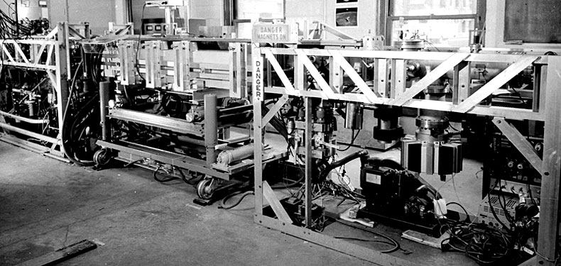
The device shown in figure 1 is a molecular-beam apparatus embodying successive oscillatory fields that has been used at Harvard for an extensive series of experiments in recent years.

Figure 1. Molecular-beam apparatus with successive oscillatory fields. The beam of molecules emerges from a small source aperture in the left third of the apparatus, is focussed there and passes through the middle third in an approximately parallel beam. It is focussed again in the right third to a small detection aperture. The separated oscillatory electric fields at the beginning and end of the middle third of the apparatus lead to resonance transitions that reduce the focussing and therefore weaken the detected beam intensity.
Let me now review the successive oscillating field method, particularly as it is applied to molecular beams, microwave spectroscopy and masers.
The method
The simplicity of the original application—measurement of nuclear magnetic moments—provides one of the best ways to explain the method of separated oscillatory fields, so my discussion will be, at first, in terms of this simple model. Extension to the more general cases is then straightforward.
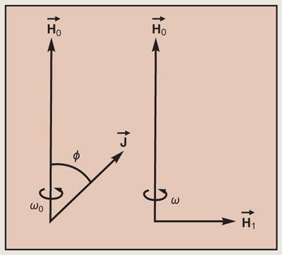
First let us remember, in outline, Rabi’s molecular-beam resonance method (figure 2). Consider classically a nucleus with spin angular momentum ℏJ and magnetic moment μ = (μ/J)J. Then in a static magnetic field H0 = H0k̂ the nucleus, due to the torque on the nuclear angular momentum, will precess like a top about H0 with the Larmor angular frequency

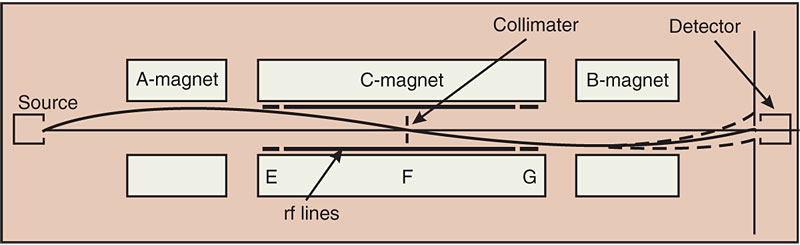
Figure 2. Molecular-beam magnetic resonance. A typical detected molecule emerges from the source, is deflected by the inhomogeneous magnetic field A, passes through the collimator and is deflected to the detector by the inhomogeneous magnetic field B. If, however, the oscillatory field in the C region induces a change in the molecular state, the B magnet will provide a different deflection and the beam will follow the dashed lines with a corresponding reduction in detected intensity. In the Rabi method the oscillatory field is applied uniformly throughout the C region as indicated by the long rf lines F, whereas in the separated oscillatory field method the rf is applied only in the regions E and G.

as shown in figure 3. Consider an additional magnetic field H1 perpendicular to H0 and rotating about it with angular frequency ω. Then, if at any time H is perpendicular to the plane of H0 and J, it will remain perpendicular to it provided ω = ω0. In that case J will also precess about H1 and the angle ϕ will continuously change in a fashion analogous to the motion of a “sleeping top”; the change of orientation can be detected by allowing the molecular beam containing the magnetic moments to pass through inhomogeneous fields as in figure 2. If ω is not equal to ω0, H will not remain perpendicular to J; so ϕ will increase for a short while and then decrease, leading to no net change. In this fashion the Larmor precession frequency ω0 can be detected by measuring the oscillator frequency ω at which there is maximum reorientation of the angular momentum. This procedure is the basis of the Rabi molecular-beam resonance method.

Figure 3. Precession of the nuclear angular momentum J (left) and the rotating magnetic field H1 (right) in the Rabi method.
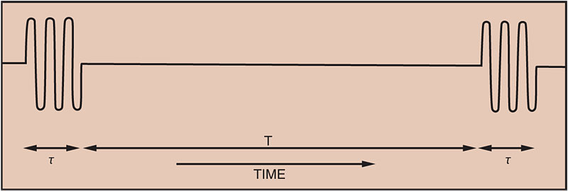
The separated oscillatory field method is much the same except that the rotating field H1 seen by the nucleus is applied initially for a short time τ, the amplitude of H1 is then reduced to zero for a relatively long time T and then increased to H1 for a time τ, with phase coherency being preserved for the oscillating fields as shown in figure 4. This can be done, for example, in a molecular-beam apparatus in which the molecules first pass through a rotating field region, then a region with no rotating field and finally a region with a second rotating field driven phase coherently by the same oscillator.

Figure 4. Two separated oscillatory fields, each acting for a time τ, with zero field acting for a time T. Phase coherency is preserved between the two oscillatory fields.
If the angular momentum is initially parallel to the fixed field (so that ϕ is equal to zero initially) it is possible to select the magnitude of the rotating field so that ϕ is π/2 radians at the end of the first oscillating region. While in the region with no oscillating field, the magnetic moment simply precesses with the Larmor frequency appropriate to the magnetic field in that region. When the magnetic moment enters the second oscillating field region there is again a torque acting to change ϕ. If the frequency of the rotating field is exactly the same as the mean Larmor frequency in the intermediate region there is no relative phase shift between the angular momentum and the rotating field.
Consequently, if the magnitude of the second rotating field and the length of time of its application are equal to those of the first region, the second rotating field has just the same effect as the first one—that is, it increases ϕ by another π/2, making ϕ = π, corresponding to a complete reversal of the direction of the angular momentum. On the other hand, if the field and the Larmor frequencies are slightly different, so that the relative phase angle between the rotating field vector and the precessing angular momentum is changed by π while the system is passing through the intermediate region, the second oscillating field has just the opposite effect to the first one; the result is that ϕ is returned to zero. If the Larmor frequency and the rotating field frequency differ by just such an amount that the relative phase shift in the intermediate region is exactly an integral multiple of 2π, ϕ will again be left at π just as at exact resonance.
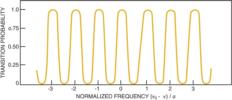
In other words if all molecules have the same velocity the transition probability would be periodic as in figure 5. However, in a molecular beam resonance experiment one can easily distinguish between exact resonance and the other cases. In the case of exact resonance the condition for no change in the relative phase of the rotating field and of the precessing angular momentum is independent of the molecular velocity. In the other cases, however, the condition for integral multiple of 2π relative phase shift is velocity dependent, because a slower molecule is in the intermediate region longer and so experiences a greater shift than a faster molecule. Consequently, for the molecular beam as a whole, the reorientations are incomplete in all except the resonance cases. Therefore, one would expect a resonance curve similar to that shown in figure 6, in which the transition probability for a particle of spin 1⁄2 is plotted as a function of frequency.

Figure 6. When the molecules have a Maxwellian velocity distribution, the transition probability is as shown by the black line for optimum rotating field amplitude. (L is the distance between oscillating field regions, α is the most probable molecular velocity and ν is the oscillator frequency.) The colored line shows the transition probability for an oscillating field of one-third strength, and the dashed line represents the single oscillating field method when the total duration is the same as the time between separated oscillatory field pulses.
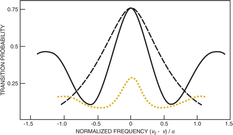

Figure 5. Transition probability that would be observed in a separated oscillatory field experiment if all the molecules in the beam had a single velocity.
From a quantum-mechanical point of view, the oscillating character of the transition probability in figures 5 and 6 is the result of the cross term CiifCiff* in the calculation of the transition probability; Ciif is the probability amplitude for the nucleus to pass through the first oscillatory field region with the initial state i unchanged but for there to be a transition to state f in the final field, whereas Ciff is the amplitude for the alternative path with the transition to the final state f being in the first field with no change in the second. The interference pattern of these cross terms for alternative paths gives the narrow oscillatory pattern of the transition probability curves in figures 5 and 6. Alternatively the pattern can in part be interpreted in terms of the Fourier analysis of an oscillating field, such as that of figure 4, which is on for a time τ, off for T and on again for τ. However, the Fourier-analysis interpretation is not fully valid since with finite rotations of J, the problem is a non-linear one.
For the general two-level system, the transition probability P for the system to undergo a transition from state i to f can be calculated quantum mechanically in the vicinity of resonance and is given 2 by

where


and where Wi is the energy of the initial state i, Wf of the final state f, and b is the amplitude of the perturbation Vif inducing the transition as defined 2 by

and the averages in (Wi − Wf) are over the intermediate region. For the special case of spin 1⁄2 and a nuclear magnetic moment, ω0 is given in equation (1) and

The results for spin 1⁄2 can be extended to higher spins by the Majorana formula. 12
If equation (2) is averaged over a Maxwellian velocity distribution the result in the vicinity of the sharp resonance is given in figure 6.
The separated oscillatory field method possesses a number of advantages, which we will discuss next.
Advantages
Among the benefits are:
‣ The resonance peaks are only 0.6 times as broad as the corresponding ones with the Rabi method and the same length of apparatus. This narrowing corresponds to the peaks in a two-slit optical interference pattern being narrower than the central diffraction peak of a single wide slit aperture whose width is equal to the separation of the slits.
‣ The sharpness of the resonance is not reduced by non-uniformities of the constant field since from both the qualitative description and from equations 2 and 5 it is only the space-average value of the energies along the beam path that is important. This advantage often permits increases in precision by a factor of 20 or more.
‣ The method is often more convenient and effective at very high frequencies where the wavelength may be comparable to the length of the region in which the energy levels are studied.
‣ Provided there is no unintended phase shift between the two oscillatory fields, first-order Doppler shifts are eliminated.
‣ The method may be applied to study energy levels in a region into which an oscillating field cannot be introduced; for example, the Larmor precession of neutrons can be measured while they are inside a magnetized iron block.
‣ The lines can be narrowed by reducing the amplitude of the rotating field below the optimum, as shown by the colored curve in figure 6. The narrowing is the result of the low amplitude favoring slower-than-average molecules.
‣ If the atomic state being studied decays spontaneously, the separated oscillatory field method permits the observation of narrower resonances than those anticipated from the lifetime and the Heisenberg uncertainty principle provided the two separated oscillatory fields are sufficiently far apart; only states that survive sufficiently long to reach the second oscillatory field can contribute to the resonance. This method, for example, has been used effectively by Francis Pipkin, Paul Jessop and Stephen Lundeen 13 in studies of the Lamb shift.
These advantages have led to the extensive use of the method in molecular and atomic-beam spectroscopy. One of the best-known of these uses is in atomic cesium standards of frequency and time.
As in any high-precision experiment, care must be exercised with the separated oscillatory field method to avoid obtaining misleading results. Ordinarily these potential distortions are more easily understood and eliminated with the separated oscillatory field method than are their counterparts in most other high-precision spectroscopy. Nevertheless the effects are important and require care in high-precision measurements. I have discussed the various effects in detail elsewhere 13 , 14 , 15 but I will summarize them here.
Precautions
Variations in the amplitudes of the oscillating fields from their optimum values may markedly change the shape of the resonance, including the replacement of a maximum transition probability by a minimum. However, symmetry about the exact resonance frequency is preserved, so no measurement error need be introduced by such amplitude variations.
14
,
15
Variations of the magnitude of the fixed field between (but not in) the oscillatory field regions do not ordinarily distort a molecular beam resonance provided the average transition frequency (Bohr frequency) between the two fields equals the values of the transition frequencies in each of the two oscillatory field regions alone. If this condition is not met, there can be some shift in the resonance frequency. 14 , 15
If, in addition to the two energy levels between which transitions are studied, there are other energy levels partially excited by the oscillatory field, there will be a pulling of the resonance frequency as in any spectroscopic study and as analyzed in detail in the literature. 13 , 14 , 15
Even in the case when only two energy levels are involved, the application of additional rotating magnetic fields at frequencies other than the resonance frequency will produce a net shift in the observed resonance frequency, as discussed elsewhere. 13 , 14 , 15 A particularly important special case is the effect identified by Felix Bloch and Arnold Siegert, 16 which occurs when oscillatory rather than rotating magnetic fields are used. Since an oscillatory field can be decomposed into two oppositely rotating fields, the counter-rotating field component automatically acts as such an extraneous rotating field. The theory of the Bloch–Siegert effect in the case of the separated oscillatory field method has been developed by Ramsey, 17 , 19 J. H. Shirley, 18 R. Fraser Code 19 and Geoffrey Greene. 20 Another example of an extraneously introduced oscillating field is that which results from the motion of an atom through a field H0 whose direction varies in the region traversed.
Unintended relative phase shifts between the two oscillatory field regions will produce a shift in the observed resonance frequency. 13 , 14 , 15 This is the most common source of possible error, and care must be taken to avoid it either by eliminating such a phase shift or by determining the shift—say by measurements with the molecular beam passing through the apparatus first in one direction and then in the opposite direction.
In some instances of closely overlapping spectral lines the subsidiary maxima associated with the separated oscillatory field method can cause confusion. Sometimes this problem can be eased by using three or four separated oscillatory fields as we shall see, but ordinarily when there is extensive overlap of resonances and the resultant envelope is to be studied, it is best to use a single oscillatory field.
Extensions of the method
Although, as we discussed above, unintended phase shifts can cause distortions of the observed resonance, it is often convenient to introduce phase shifts deliberately to modify the resonance shape.
21
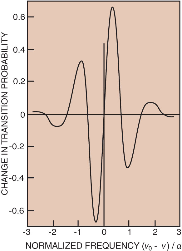
Thus, if the change in transition probability is observed when the relative phase is shifted from + π/2 to − π/2 one sees a dispersion curve shape
21
as in figure 7. A resonance with the shape of figure 7 provides maximum sensitivity for detecting small shifts in the resonance frequency, say by applying an external electric field.

Figure 7. Theoretical change in transition probability on reversing a π/2 phase shift. This resonance shape gives the maximum sensitivity by which to detect small shifts in the resonance frequency.
For most purposes the highest precision can be obtained with just two oscillatory fields separated by the maximum time, but in some cases it is better to use more than two separated oscillatory fields. 4 The theoretical resonance shapes with two, three, four and infinitely many oscillatory fields are given in figure 8. The infinitely many oscillatory field case, of course, by definition becomes the same as the single long oscillatory field if the total length of the transition region is kept the same and the infinitely many oscillatory fields fill in the transition region continuously as we assumed in figure 8. For many purposes this is the best way to think of the single oscillatory field method, and this point of view makes it apparent that the single oscillatory field method is subjected to complicated versions of all the distortions discussed in the previous section. It is noteworthy that, as the number of oscillatory field regions is increased for the same total length of apparatus, the resonance width is broadened; the narrowest resonance is obtained with just two oscillatory fields separated the maximum distance apart. Despite this advantage, there are valid circumstances for using more than two oscillatory fields. With three oscillatory fields the first and largest side lobe is suppressed, which may help in resolving two nearby resonances; for a larger number of oscillatory fields additional side lobes are suppressed, and in the limiting case of a single oscillatory field there are no sidelobes. Another reason for using a large number of successive pulses can be the impossibility of obtaining sufficient power in a single pulse to induce adequate transition probability with a small number of pulses.

Figure 8. Multiple oscillatory fields. The curves show molecular-beam resonances with two, three, four and infinitely many successive oscillating fields. The case with an infinite number of fields is equivalent to a single oscillating field extending throughout the entire region.

The earliest use of the successive oscillatory field method involved two oscillatory fields separated in space, but it was early realized that the method with modest modifications could be applied to the separations being in time, say by the use of coherent pulses. 4
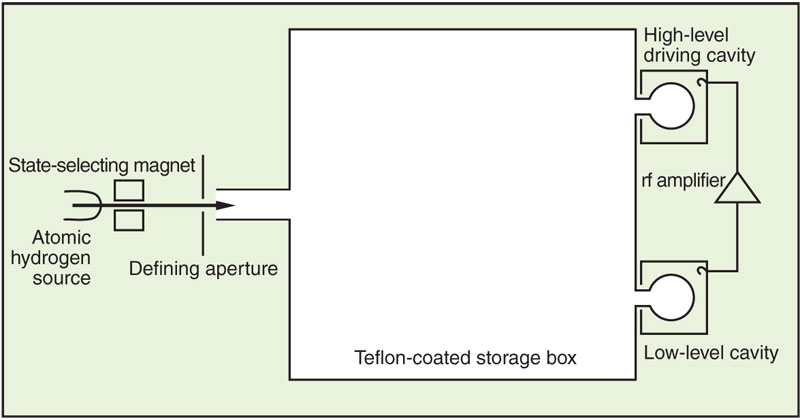
If more than two successive oscillatory fields are utilized it is not necessary to the success of the method that they be equally spaced in time; 4 the only requirement is that the oscillating fields be coherent—as is the case if the oscillatory fields are all derived from a single continuously running oscillator. In particular, the separation of the pulses can even be random, 4 as in the case of the large box hydrogen maser 22 shown in figure 9. The atoms being stimulated to emit move randomly into and out of the cavities with oscillatory fields and spend the intermediate time in the large container with no such fields.

Figure 9. A large box hydrogen maser shown schematically. The two cavities on the right constitute two separated oscillatory fields; atoms move randomly in and out of these cavities but spend the greater part of their time in the large field-free container.
The full generalization of the successive oscillatory field method is excitation by one or more oscillatory fields that vary arbitrarily with time in both amplitude and phase. 5
More recent modifications of the successive oscillatory field method include the following three applications.
V. F. Ezhov and his colleagues, 23 in a neutron-beam experiment, used an inhomogeneous static field in the region of each oscillatory field region such that initially when the oscillatory field is applied conditions are far from resonance. Then, when the resonance condition is slowly approached, the magnetic moment that was originally aligned parallel to H0 will adiabatically follow the effective magnetic field on a coordinate system rotating with H1 until at the end of the first oscillatory field region the moment is parallel to H1 and thereby at angle ϕ = π/2. As in the ordinary separated oscillatory field experiment, the moment precesses in the intermediate region, and the phase of the precession relative to that of the oscillator is detected in the final region by an arrangement where the fields are such that the effective field in the rotating coordinate system shifts from parallel to H1 to parallel to H0. This arrangement has the theoretical advantage that the maximum transition probability can be unity even with a velocity distribution, and the resonance is less dependent on the value of the field in the oscillatory field region. On the other hand, the method may be less well adapted to the study of complicated spectra, and it requires a special nonuniform magnetic field.
I emphasized in an earlier section that one of the principal sources of error in the separated oscillatory field method is that which arises from uncertainty in the exact value of the relative phase shift in the two oscillatory fields. David Wineland, Helmut Hellwig and Stephen Jarvis 24 have pointed out that this problem can be overcome with a slight loss in resolution by driving the two cavities at slightly different frequencies so that there is a continual change in the relative phase. In this case the observed resonance pattern will change continuously from absorption to dispersion shape. The envelope of these patterns, however, can be observed and the position of the maximum of the envelope is unaffected by relative phase shifts. Since the envelope is about twice the width of a specific resonance there is some loss of resolution in this method, but in certain cases this loss may be outweighed by the freedom from phase-shift errors.
Finally, the extension of the method to laser spectroscopy has aroused a great deal of interest. These applications of course require some modifications from the form of the technique most widely applied to molecular beams, 6–10 due to differences in wavelengths, state lifetimes and so on. However, the necessary modifications have been made and the method continues to be of real value in laser spectroscopy—particularly in cases where the extra effort required is justified by the need for multiple pulses or high precision.
Advice from Rabi
The first advice I received from Rabi in 1937 when I applied to him to begin my research was that I should not go into the field of molecular beams since the interesting problems amenable to that technique had already been solved and there was little future to the field. I have often wondered how I . . . had the temerity to disregard this bit of advice from the master. However, I am grateful that I did since the advice was given only a few months before Rabi’s great invention of the molecular beam resonance method . . . which led to such fundamental discoveries as the quadrupole moment of the deuteron, the Lamb shift, the anomalous magnetic moment of the electron and [to] numerous other discoveries and measurements.
(Quoted from Norman Ramsey’s contribution to A Tribute to Professor I. I. Rabi, Columbia University, New York, 1970.)
This article is an adaptation of a paper presented at the Tenth International Quantum Electronics Conference, held in Atlanta, Georgia, in May 1978.
References
1. N. F. Ramsey, Phys. Rev. 76, 996 (1949). https://doi.org/10.1103/PhysRev.76.996
2. N. F. Ramsey, Phys. Rev. 78, 695 (1950). https://doi.org/10.1103/PhysRev.78.695
3. N. F. Ramsey, H. B. Silsbee, Phys. Rev. 84, 506 (1951). https://doi.org/10.1103/PhysRev.84.506
4. N. F. Ramsey, Rev. Sci. Instr. 28, 57 (1957). https://doi.org/10.1063/1.1715708
5. N. F. Ramsey, Phys. Rev. 109, 822 (1958). https://doi.org/10.1103/PhysRev.109.822
6. Y. V. Baklanov, B. V. Dubetsky, V. B. Chebotsev, Appl. Phys. 9, 171 (1976). https://doi.org/10.1007/BF00903955 and
Y. V. Baklanov, B. V. Dubetsky, V. B. Chebotsev, Appl. Phys. 11, 201 (1976). https://doi.org/10.1007/BF009206077. J. C. Bergquist, S. A. Lee, J. L. Hall, Phys. Rev. Lett. 38, 159 (1977) https://doi.org/10.1103/PhysRevLett.38.159 and
J. C. Bergquist, S. A. Lee, J. L. Hall, Laser Spectroscopy III, 142 (1978).8. M. M. Salour, C. Cohen-Tannoudji, Phys. Rev. Lett. 38, 757 (1977) https://doi.org/10.1103/PhysRevLett.38.757 ,
M. M. Salour, C. Cohen-Tannoudji, Laser Spectroscopy III, 135 (1978),
Appl. Phys. 15, 119 (1978) and
M. M. Salour, C. Cohen-Tannoudji, Phys. Rev. A17, 614 (1978).9. C. J. Bordé, C. R. Acad. Sci. Paris 284B, 101 (1977).
10. T. W. Hänsch, Laser Spectroscopy III, 149 (1978).
11. V. P. Chebotayev, A. V. Shishayev, B. Y. Yurshin, L. S. Vasilenko, N. M. Dyuba, M. I. Skortsov, Appl. Phys. 15, 43, (1987) https://doi.org/10.1007/BF00896888 ,
V. P. Chebotayev, A. V. Shishayev, B. Y. Yurshin, L. S. Vasilenko, N. M. Dyuba, M. I. Skortsov, Appl. Phys. 15, 219 (1987) https://doi.org/10.1007/BF00928212 and
V. P. Chebotayev, A. V. Shishayev, B. Y. Yurshin, L. S. Vasilenko, N. M. Dyuba, M. I. Skortsov, Appl. Phys. 15, 319 (1987).https://doi.org/10.1007/BF0089611512. S. R. Lundeen, P. E. Jessop, F. M. Pipkin, Phys. Rev. Lett. 34, 377 (1975) https://doi.org/10.1103/PhysRevLett.34.377 and
S. R. Lundeen, P. E. Jessop, F. M. Pipkin, Phys. Rev. Lett. 34, 1368 (1975) https://doi.org/10.1103/PhysRevLett.34.1368 .13. N. F. Ramsey, Molecular Beams, Oxford University Press (1956).
14. N. F. Ramsey, Le Journal de Physique et Radium 19, 809 (1958).
15. N. F. Ramsey, in Recent Research in Molecular Beams (I. Estermann, ed.) Academic Press, New York (1958), page 107.
16. F. Bloch, A. Siegert, Phys. Rev. 57, 522 (1940). https://doi.org/10.1103/PhysRev.57.522
17. N. F. Ramsey, Phys. Rev. 100, 1191 (1955). https://doi.org/10.1103/PhysRev.100.1191
18. J. H. Shirley, J. Appl. Phys. 34, 783 (1963). https://doi.org/10.1063/1.1729536
19. R. F. Code, N. F. Ramsey, Phys. Rev. A4, 1945 (1971).
20. G. Greene, Phys. Rev. A18, 1057 (1978).
21. N. F. Ramsey, H. B. Silsbee, Phys. Rev. 84, 506 (1951). https://doi.org/10.1103/PhysRev.84.506
22. E. E. Uzgiris, N. F. Ramsey, Phys. Rev. A1, 429 (1970).
23. V. F. Ezhov, S. N. Ivanov, I. M. Lobashov, V. A. Nazarenko, G. D. Porsev, A. P. Serebrov, R. R. Toldaev, Sov. Phys.-JETP Lett. 24, 39 (1976).
24. S. Jarvis Jr., D. J. Wineland, H. Hellwig, J. Appl. Phys. 48, 5336 (1977). https://doi.org/10.1063/1.323567
More about the authors
Norman F. Ramsey is Higgins Professor of Physics at Harvard University.


