The dichotomous history of diffusion
DOI: 10.1063/1.3177228
Diffusion implies spreading, either observable (physical), or abstract and probabilistic (stochastic). At the beginning of the 19th century, the mathematics of both were established by Joseph Fourier and Pierre Simon Laplace. In 1807 Fourier submitted a monograph, Théorie de la propagation de la chaleur dans les solides (Theory of the propagation of heat in solids), to the French Academy of Sciences and introduced the partial differential equation describing heat flow. 1 , 2 The academy appointed Joseph Lagrange and Laplace as two of the four reviewers of the monograph; they questioned Fourier’s use of trigonometric series to solve the heat equation. Hence, the work was never approved.
At the time, Laplace was working on his theory of probability—in particular, estimating the probability that the sum of n random variables may be equal to or less than a certain value when n is very large. In 1809 he formulated a partial differential equation with the same form as Fourier’s heat equation, whose solution would provide an estimate of the probability. 3 Soon thereafter, Laplace published Théorie analytique des probabilités (Analytical theory of probability) 4 and Fourier published Théorie analytique de la chaleur (Analytical theory of heat). 5
Fourier’s theory had an immediate impact on mathematical physics by opening up new avenues for the study of heat. It also inspired scientists of the day to apply the diffusion model to electricity, molecules, and fluid flow in resistive media. However, Laplace’s stochastic diffusion, based on his probability studies, went largely unnoticed for decades. Toward the close of the 19th century, Lord Rayleigh 6 , 7 and economist and statistician Francis Edgeworth 8 drew on Laplace’s treatise on probability theory to formulate the stochastic diffusion equation with probability density as the dependent variable. Shortly thereafter, Louis Bachelier 9 formulated a diffusion equation to model random price fluctuations in the stock market. At the turn of the 20th century, mathematics of diffusion had established two separate identities—one as a physically observable process, the other as a probabilistic description.
In 1905 Albert Einstein recognized the equivalence between two diffusion coefficients—one describing random events, the other describing a physical process—and used that equivalence to experimentally establish a kinetic theory of heat based on molecular motion and estimate Avogadro’s number, a quantity of fundamental importance in chemistry. 10
The diffusion equation is widely used in physical, biological, geological, and social sciences in physical or stochastic form. Commonly, mathematicians and scientists focus attention on the similarity of mathematical patterns in applying the diffusion model to one field or another and ignore the inherent differences in the nature of the processes. Nevertheless, the differences between physical and stochastic diffusion are as notable as their similarities. In his investigations, Fourier was inspired by curiosity to comprehend the role of heat in Earth’s lithosphere, oceans, and atmosphere. He thus found it surprising that mathematical results bearing on physical diffusion were also relevant to problems in the abstract theory of probability. 5
To provide insight into diverse phenomena and the evolution of the mathematical ideas, this paper traces the twofold history of diffusion.
Birth of the concepts
Soon after his return from the Egyptian campaign in 1801, Napoleon Bonaparte appointed Fourier as prefect of the Department of Isère, whose headquarters were in Grenoble. Despite major administrative responsibilities, Fourier embarked on developing a theory for heat that would be as profound as that of rational mechanics, which dominated post-Newton thought. Combining action at a distance, an idea central to celestial mechanics, and Newton’s law of cooling—the rate at which a body loses heat is proportional to the temperature difference with its surroundings—Fourier attempted to formulate a differential equation for heat conduction, but he met with mathematical difficulties. 2 He soon abandoned action at a distance and began visualizing solids as continuous media in which heat propagated by conduction. 1 He also went beyond Newton’s law of cooling and proposed that the rate of heat transfer between two points in a solid is proportional to their temperature difference and inversely proportional to their distance. He then formally defined thermal conductivity, which when multiplied by the temperature gradient at a point yields the heat flux per unit area per unit time in the direction of the gradient.
In his 1807 monograph, Fourier introduced the parabolic partial differential equation in three dimensions, 2
where T is temperature; t time; K thermal conductivity; C specific heat; D density of the solid; and x, y, and z spatial coordinates. To solve his equation, Fourier chose solid, symmetrical bodies with well-defined bounding surfaces—a prism, rod, cube, cylinder, or sphere. Temperatures or fluxes were prescribed on the bounding surfaces, and initial conditions were specified at every point in the interior. Fourier recognized that thermal conductivity and specific heat would generally vary with temperature. However, such variation would render the equation nonlinear and intractable. Therefore, he assumed that the dependence of K and C on T could be reasonably ignored over small temperature ranges, which renders the equation linear and amenable to solution by algebraic methods. Among the methods he devised to solve the equation, the superposition of trigonometric series was of fundamental interest in mathematical analysis.

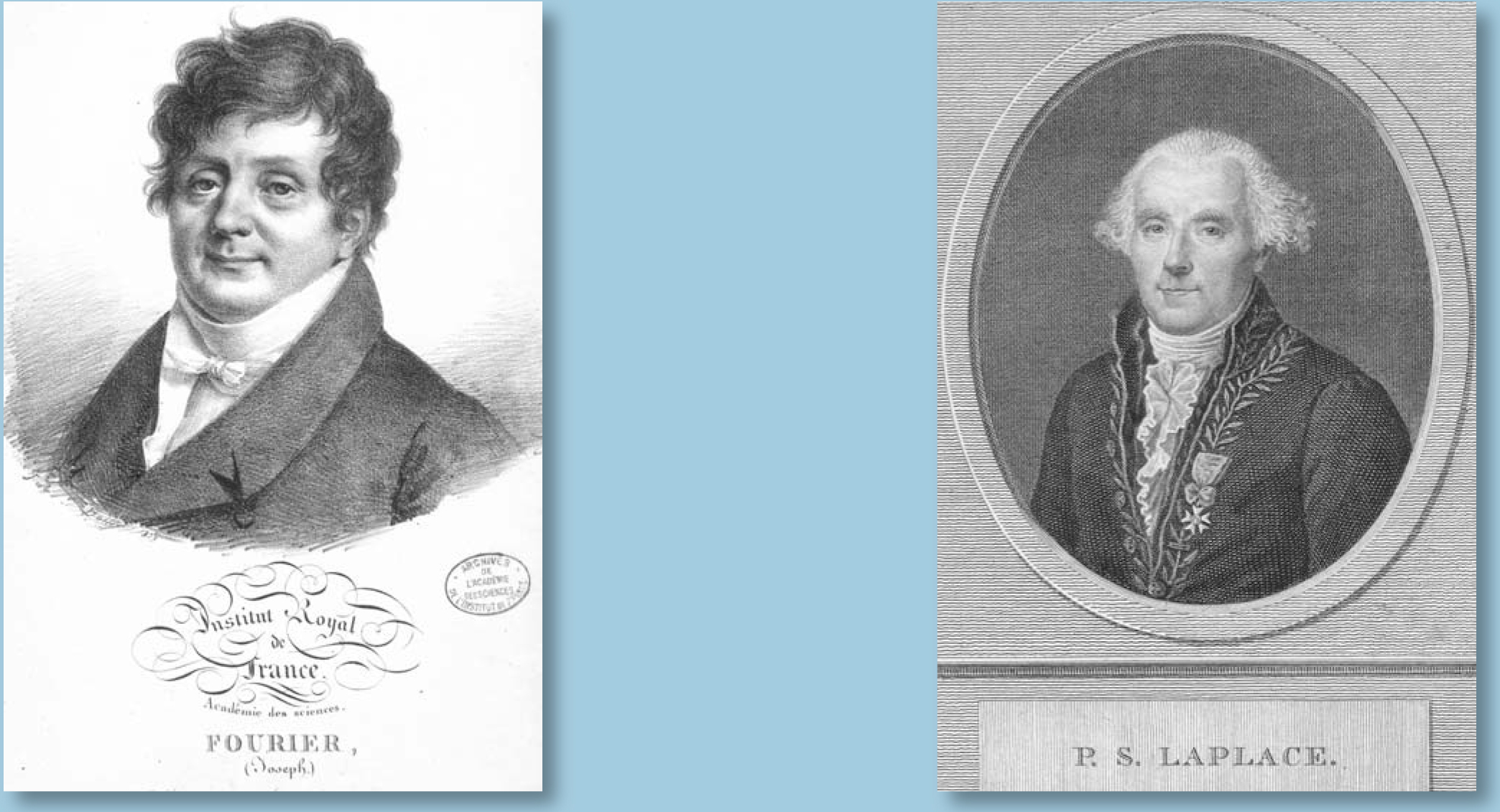
Joseph Fourier (1768–1830, left) and Pierre Simon Laplace (1749–1827, right). Fourier’s heat equation of 1807 probably influenced Laplace to express as a partial differential equation the partial difference equation that he had already derived for the behavior of random variables. In turn, Laplace inspired Fourier to extend the heat equation to diffusion in infinite domains.
(Portraits courtesy of Académie des sciences, Institut de France.)
At the time, Laplace had just completed publication of Traité de mécanique céleste (Treatise on celestial mechanics), which had occupied a better part of the previous 20 years, and resumed work on probability theory, particularly concerning the probability that the sum of a large number of identically distributed random variables would take on a given value. It was known through earlier investigations by Jacques Bernoulli, Abraham de Moivre, and others that the probability would be the coefficient of a particular term in a power series.
Unfortunately, estimating the numerical magnitude of the coefficient was difficult when the number of summed random variables became very large. One way to overcome that difficulty was to evaluate the coefficient as a definite integral. Accordingly, Laplace used “génératrice” functions to set up partial difference equations with the coefficient of interest as the dependent variable. 3 In particular, he applied a génératrice function to a power series involving the product of two terms (tx tx’ , where t is arbitrary) with coefficient yx,x’ , and obtained the partial difference equation,
where Δ2 yx,x′ = yx+2,x’ − 2yx+1,x’ + yx,x′ and Δ’yx,x′ = yx,x′+1 − yx,x′ . Here subscripts x and x’ are integers. As the number of terms in the power series becomes very large, the difference equation can be replaced by its differential equivalent (in Laplace’s notation):
In this equation, yx,x’ , represents the probability that the sum of x’ identically distributed random variables takes on the value x. Compared to the heat equation, probability y corresponds to temperature; the magnitude of the sum of random variables, x, corresponds to distance; and the number of random variables, x’, corresponds to time. Laplace then demonstrated that
where φ is any arbitrary function, satisfies equation
In equation
The French Academy of Sciences instituted a prize competition in 1811 on the topic of heat conduction. Fourier submitted an extended version of his rejected 1807 work and was awarded the prize in 1812. Probably influenced by Laplace, Fourier had extended his studies in the prize essay to infinite domains, within which diffusion was driven purely by initial conditions. He considered an infinite line with −∞ < x < +∞. At time t = 0, the temperature everywhere along the line was zero, except over a segment extending on either side of x = 0. Over that segment, the temperature distribution was an arbitrarily prescribed function f(x). To solve for T(x,t), Fourier sought solutions in the form T = e−x e-kt and showed through a series of transformations that equation
Going beyond génératrice functions, Laplace was more concerned with obtaining a mathematical proof of what is now known as the central limit theorem. Of fundamental importance in probability theory, the theorem states that the sum of n independently and identically distributed random variables x 1, x 2, x 3, … xn with mean µ and variance σ2 asymptotically approaches a normal distribution with mean nµ and variance nσ2:
Laplace succeeded in providing the proof for variables of arbitrary distribution. 13
In his 1822 Théorie analytique de la chaleur, 5 Fourier went further with infinite domains than he had in the prize essay. For example, he imagined the infinite line as having a certain quantity of heat released within a very small segment ω located at x = 0 at t = 0 such that its temperature increases to a value f. Everywhere else the temperature remains 0. That condition is referred to as an instantaneous plane source. The differential equation for that one-dimensional problem is satisfied by
where ωf is the strength of the source and η = K/CD is thermal diffusivity. If we let ωf = 1 in equation
Random walk through the 19th century
The first phase in the history of diffusion came to an end with Fourier’s 1822 treatise. Over succeeding decades, Fourier’s physical diffusion equation (equation
Fourier’s analysis of trigonometric series led to much interest in precisely and rigorously defining functions of real variables through the contributions of Lejeune Dirichlet and Bernhard Riemann. 11 On the experimental side, Thomas Graham’s investigations on gas diffusion and Adolph Fick’s studies on liquid diffusion showed that material diffusion involves simultaneous transport of two or more species in opposite directions, whereas thermal diffusion involves only one migrating species, heat. 14
In 1887 Jacobus van’t Hoff examined data on osmotic pressure exerted by nonelectrolytes in aqueous solutions and discovered that the relations among osmotic pressure, solution volume, and temperature were remarkably similar to ideal gas laws. 15 He postulated that osmotic pressure is a manifestation of kinetic energy of solute molecules per unit volume of solution and that osmotic pressure depends on the number of molecules, regardless of their type. Soon afterward, Walther Nernst gave a dynamical interpretation of Fick’s law. 16 He suggested that molecular diffusion was governed by the gradient of osmotic pressure and that in dilute solutions, concentration and osmotic pressure were mutually related by a simple constant.
Through much of the 19th century, scientists debated the molecular nature of matter. Toward the end of the century, additional evidence in favor of molecular makeup of matter was emerging from experimental observations on Brownian motion; those observations suggested that thermal agitation of molecules was its underlying cause.
Stochastic diffusion and physical diffusion are unified by analogous expressions,
in which the variance—that is, statistical dispersion—is analogous to diffusivity, and the number of random variables summed up is analogous to time. The unity of those equations was rediscovered in the 1880s by Rayleigh and Edgeworth. Rayleigh addressed the probability associated with a large number of vibrations of the same amplitude with phases either positive or negative. 6 For that distribution of vibrations, the variance is unity. A more general problem involving the sum of random variables had been solved by Laplace using Bernoulli’s theorem. 4 Let the sum of n random variables chosen from the distribution be x. Rayleigh showed that the probability density function for the vibration problem is
which is a consequence of the central limit theorem. More than a decade later, Rayleigh recognized serendipitously that the probability density function is also a solution to Fourier’s diffusion equation. 7 Let f(n,x) be the probability that the sum of n random variables equals x; the evolution of that probability as a function of x and n is given by the partial differential equation
where ½ represents the diffusion coefficient, which is equal to half of the variance. Rayleigh also showed that the average intensity—or, more precisely, the expectation value for the square of the amplitude—is equal to n.
Edgeworth, a statistician, approached the problem of error propagation with the premise that every measurable observation may be regarded as a function of an indefinite number of elements, each being a member of the same symmetrical frequency distribution.
8
He set himself the task of showing that when the number of elements is large, the cumulative error approaches a normal distribution, a result known as the law of error. To that end he followed Laplace’s approach, assuming that the required function is a particular term in a power series. Using a recursive relationship, he then showed that the function representing cumulative error is obtainable from the solution to a partial differential equation of the same form as equation
Rayleigh and Edgeworth firmly established Laplace’s stochastic diffusion equation as a description of the evolution of a normal distribution with increasing sample size. Still, their analyses had been restricted to thought experiments involving random samples, not physical observations. The first step toward addressing time was taken by Bachelier, who developed a theory of speculation, and Karl Pearson, who introduced the phrase “random walk.”
Bachelier showed that a diffusion equation could describe temporal variations in the values of stock option prices, provided one first make some assumptions about the randomness of stock prices.
9
By pursuing an approach similar to Rayleigh’s involving finite difference equations,
7
he introduced the notion of “radiation of probability,” which is conceptually analogous to Fourier’s law of heat conduction. Bachelier expressed the time evolution of stock price in the form of a diffusion equation similar to equation
Pearson’s contribution came in the form of a short letter to the readers of Nature
17
in 1905. He sought help solving the following problem: A man starts from O and walks ℓ yards in a straight line; he then turns through some angle and walks another ℓ yards in a straight line, a process he repeats n times. What is the probability that after n stretches, he ends up at a distance between r and r + δr from O? Rayleigh responded to the letter by drawing attention to his solution (equation
A synthesis
That same year, Einstein filed his dissertation on determining molecular dimensions by studying the diffusion of sugar, a non-electrolyte, in aqueous solutions. He then devised an experimental methodology to establish a molecular-kinetic theory of heat. His premise was that if the theory were correct, then microscopically visible particles in suspension must perform random movements of sufficient magnitude to be visually observable. Moreover, he asserted that if his theory could be experimentally validated, classical thermodynamics would be inapplicable to microscopically distinguishable particles.

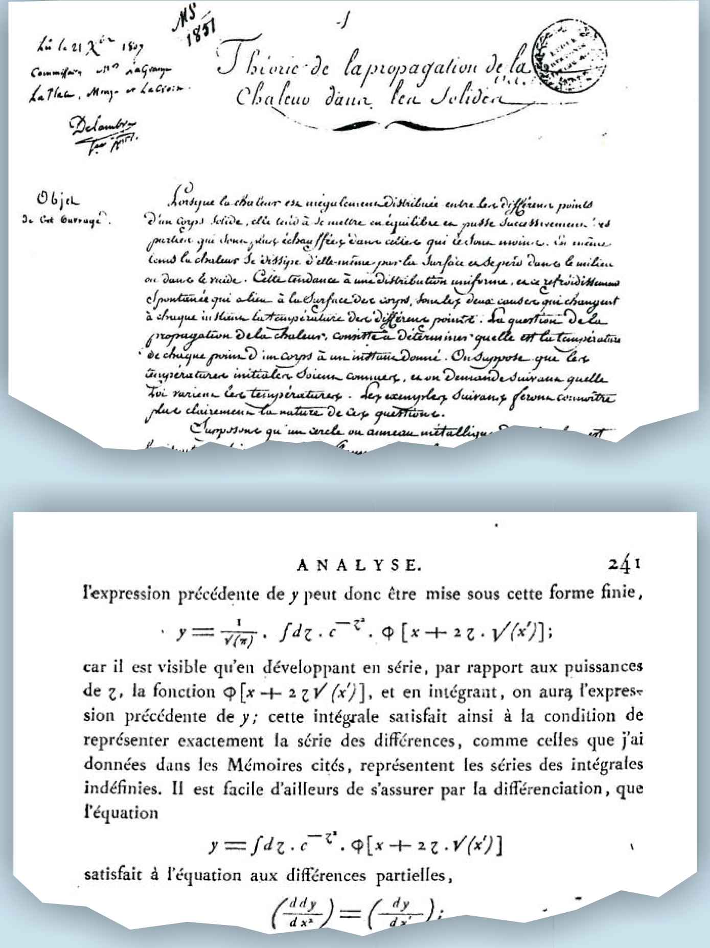
Joseph Fourier’s monograph on heat diffusion was submitted handwritten (top) to the Institut de France in 1807. Among the four referees were Joseph Lagrange and Pierre Simon Laplace, who rejected the monograph out of mistrust of Fourier’s use of trigonometric series. It was never published. Laplace expressed probabilities associated with random variables as partial difference equations as early as 1779. This 1809 excerpt (bottom) from Journal de I’École Polytechnique shows his solution to a partial differential equation analogous to the heat equation.
Einstein’s approach consisted in looking at particle motion on both a macroscale and a microscale, 10 for both of which the driving force on the particles would come from the kinetic energy of solvent molecules. On the macroscale, the kinetic energy would be manifest as osmotic force, and on the microscale, as force acting randomly on individual particles. The microscale motion would be described by a stochastic diffusion equation; that on the macroscale would be expressed by the equation for molecular diffusion.
The starting point for a macroscopic description was van’t Hoff’s expression for osmotic pressure exerted by n molecules of a dilute nonelectrolyte, 15
where R is the universal gas constant, T is absolute temperature, V is solution volume, and N is Avogadro’s number. Einstein reasoned that this expression for invisible molecules was equally applicable to microscopically visible particles in suspension. He then took Nernst’s dynamical view 16 of Fick’s model for molecular diffusion and assumed that the diffusion is driven by spatial variations in osmotic pressure of the solute.
Based on those assumptions, Einstein considered a tube of uniform cross section that was filled with a dilute suspension of spherical particles of radius r, diffusing at a constant rate and driven by the difference in osmotic pressure between the two ends. The need to balance impelling osmotic forces and resistive viscous forces led him to the macroscopic, or physical, diffusion coefficient
where µ is the coefficient of viscosity.
For the microscale random walk of particles along an infinite line with origin at x = 0, he followed a recursive procedure similar to that of Edgeworth 8 and arrived at the stochastic equation
where f(x,t) is the probability that a particle would be at a distance x from the origin at time t. D s is half the variance of the distribution that describes the random motion. The equation is essentially the same as Rayleigh’s stochastic equation, equation
Assuming an equivalence between the microscopic and macroscopic representations, Dp can be treated as equal to Ds , and
Thus if λ x can be discerned from visual observations, then equation

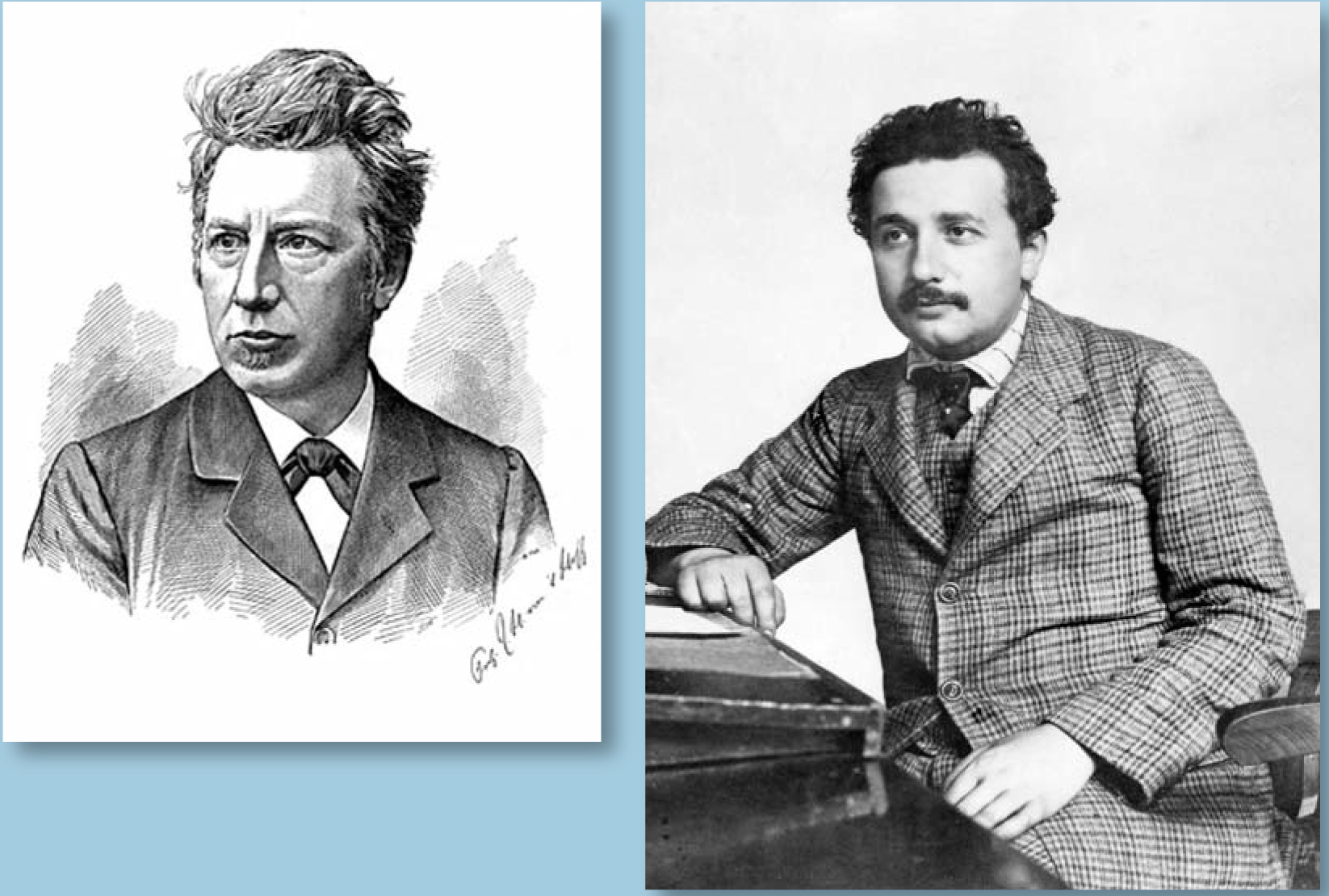
Jacobus van’t Hoff (1852-1911, left) discovered in 1887 that the behavior of osmotic pressure in dilute solutions conformed remarkably to the ideal gas laws. The conformity led him to suggest that osmotic pressure is a manifestation of kinetic energy of solute molecules and could be explained purely on the basis of the number of dissolved molecules rather than of the type of molecule. In formulating a molecular-kinetic theory of heat, Albert Einstein (1879–1955, right) used van’t Hoff’s model to cast Fick’s law of molecular diffusion in a dynamical form and derived an expression for the molecular diffusion coefficient.
(Einstein image from the Hebrew University of Jerusalem, Albert Einstein Archives, courtesy of the AIP Emilio Segrè Visual Archives.)
The stochastic diffusion equation and its solution were already well established in 1905. So also were Fick’s law for molecular diffusion and the nature of osmotic pressure. Yet Einstein’s work on Brownian motion is recognized as one of his most significant contributions. What is notable about Einstein’s work is that he looked at molecular diffusion both on the microscale as a stochastic problem and on the macroscale as a dynamical, deterministic problem. Then, with remarkable insight, he treated the two diffusion coefficients as mutually interchangeable. The result was to integrate the physical and the abstract facets of diffusion and help resolve a major problem of 19th century physics—molecular reality.
Mathematical metaphor
As the history of diffusion suggests, the evolution of ideas about it has been spurred as much by conceptualization of physical spreading (of heat and molecules, for example) as by abstract mathematical notions such as probability. But the overlap between physical and stochastic diffusion—or rather, the realm in which both models are equivalent—is limited to a narrow class of problems. To appreciate problems outside the overlap, one must strike a balance between physical intuition and mathematical abstraction.
Two physical quantities, thermal conductivity and specific heat, determine the manner in which heat spreads in a solid over time. And both can be independently measured. In stochastic diffusion, by comparison, spreading is governed by a single parameter, the variance. Although variance is mathematically analogous to thermal diffusivity—conductivity divided by specific heat—the stochastic problem has no attributes that are separately analogous to conductivity and specific heat.
The stochastic diffusion equation, as addressed by Laplace, Rayleigh, Edgeworth, Bachelier, and Einstein, is deeply connected to the central limit theorem. It is a parabolic partial differential equation in which the derivative with respect to number of samples n or time t has to be greater than zero. That is, the stochastic equation does not apply to a steady-state case in which the probability density remains constant.
In physical diffusion, by comparison, the time derivative can be zero or greater. In fact, boundary-value problems arise only when the time derivative is zero. Those problems involve steady-state spatial distributions of potentials dictated by prescribed boundary conditions or the presence of sources and sinks. Recall that Fourier’s trigonometric series solutions were restricted to bounded domains; a normal distribution pertaining to an infinite domain could not be represented by a trigonometric series. The difference suggests that the stochastic equation does not strictly apply to boundary-value problems.
Stochastic diffusion is designed to handle discrete objects that move randomly—for example, molecules diffusing in gases, liquids, or solids. However, some problems of physical diffusion are not associated with random motion. Heat is a good example. Another is the viscous motion of fluids in porous materials. Viscous motion, which involves effects of molecular collisions with the walls of a container, does not constitute molecular diffusion.
In physical diffusion, conservation of mass or energy is implicit in the partial differential equation. The dependent variable is a potential whose spatial gradient is a driving force. The slope of the curve relating potential to mass or energy is a capacitance—specific heat, for example. In stochastic diffusion, probability density is mathematically analogous to the potential of physical diffusion. That similarity, however, is superficial. Probability in stochastic diffusion denotes the number of outcomes in an interval of a histogram or the number of particles in an interval of space, expressed as a fraction of total number of outcomes or particles. Whereas a potential is defined as energy per unit mass or volume of a material, probability is not restricted to a unit interval. In stochastic diffusion, the total number of outcomes is to be held constant, or conserved, so that the definition of probability remains consistent as n is increased. In physical diffusion, the definition of potential is independent of total mass or energy of the system.
In science, metaphor plays an important role in transferring ideas among different disciplines. Metaphors, though, can often mask inner truths. Essential to scientific training is an ability to properly appreciate metaphors so that they do not inhibit a deeper understanding of phenomena. The metaphor of diffusion, which unites physical and probabilistic spreading, lucidly illustrates the power and the limitation of scientific metaphors.
I thank Jean-Pierre Kahane for insightful discussions on the mathematics and history associated with Fourier’s magnum opus. Nic Spycher helped generously with the French translation. I also greatly appreciate the library system of the University of California.
References
1. J. B.J. Fourier, Théorie de la propagation de la chaleur dans les solides, manuscript submitted to the Institut de France 21 December 1807 and archived at the library of the École Nationale des Ponts et Chaussées, Paris (1807).
2. I. Grattan-Guinness, J. R. Ravetz, Joseph Fourier, 1768–1830, MIT Press, Cambridge, MA (1972).
3. P. S. Laplace, J. Ec. Polytech. 8, 235 (1809).
For Laplace’s earlier introduction of génératrice functions, see Oeuvres complètes de Laplace, vol. 10, Gauthier-Villars, Paris (1894) p. 1
(reprinted from Mem. Acad. R. Sci. Paris, 1779, 1782).4. P. S. Laplace, Théorie analytique des probabilités, Ve Courcier, Paris (1812).
5. J. B.J. Fourier, Théorie analytique de la chaleur, Firmin Didot, Paris (1822);
see also The Analytical Theory of Heat, A. Freeman, trans., Cambridge U. Press, Cambridge, UK (1878) pp. 7–377.6. J. W. Strutt ( Lord Rayleigh ), Philos. Mag. 10, 73 (1880). https://doi.org/10.1080/14786448008626893
7. J. W. Strutt ( Lord Rayleigh ), The Theory of Sound, 2nd ed., vol. 1, MacMillan, New York (1894).
8. F. Y. Edgeworth, Philos. Mag. 16, 300 (1883). https://doi.org/10.1080/14786448308627433
9. L. Bachelier, Théorie de la spéculation, Gauthier-Villars, Paris (1900).
Eng. trans. in The Random Character of Stock Market Prices, P. H. Cootner, ed., MIT Press, Cambridge, MA (1964) p. 17.10. A. Einstein, Investigations on the Theory of the Brownian Movement, R. Fürth, ed., A. D. Cowper, trans., Methuen, London 1926
(reprinted from Ann. Phys. [Leipzig] 322, 549 [1905]).https://doi.org/10.1002/andp.1905322080611. J.-P Kahane, Proceedings of Symposia in Pure Mathematics, vol. 79, D. Mitrea, M. Mitrea, eds., American Mathematical Society, Providence, RI (2008), p. 187.
12. J. B.J. Fourier, Mem. Acad. R. Sci. Paris 4, 185 (1824);
5, 153 (1826).13. A. Hald, A History of Mathematical Statistics from 1750 to 1930, Wiley, New York (1998), p. 310.
14. T. N. Narasimhan, Rev. Geophys. 37, 151 (1999). https://doi.org/10.1029/1998RG900006
15. J. H. van’t Hoff, Z. Phys. Chem. 1, 481 (1887).
16. W. H. Nernst, Z. Phys. Chem. 2, 613 (1888).
17. K. Pearson, Nature 72, 294 (1905). https://doi.org/10.1038/072294b0
More about the authors
T. N. Narasimhan is an emeritus professor in the department of materials science and engineering and the department of environmental science, policy, and management at the University of California, Berkeley.
T. N. Narasimhan, University of California, Berkeley, US .


