Special Issue: The Kuiper Belt
DOI: 10.1063/1.1752422
On 10 January 1992, a freighter en route from Hong Kong to Tacoma, Washington, got caught in a storm in the northern Pacific Ocean, and shipping containers filled with 29 000 plastic bathtub toys were lost overboard. Ten months later, brightly colored ducks, turtles, beavers, and frogs began showing up on beaches all along the coast of Alaska. Seattle-based oceanographers Curtis Ebbesmeyer and James Ingraham quickly realized that they had a massive inadvertent experiment on their hands. In their research, the two had been studying wind and sea circulation in the northwest Pacific by systematically dropping small numbers of labeled floats from fixed locations and hoping for their recovery. As they well knew, scientists understood the physics behind the winds and currents, but the large numbers of different interactions that occur made precise prediction difficult—even with the help of large computer models. The bathtub toys provided a windfall of data that would allow the two oceanographers to chart out winds and currents and understand the complex interactions in more detail than was previously possible with their more limited data.
Like oceanographers trying with a paucity of observations to understand the complexities of currents, astronomers studying the formation and evolution of the outer Solar System have had, until recently, few data points around which to spin their theories. The outer Solar System’s four giant planets were each created and moved around by a complex suite of interactions. Trying to piece together all of those interactions to discern a history would be like trying to use just four large shipwrecks washed ashore to understand the flows of all of the oceans’ currents.
The breakthrough for astronomers came a few months before the first plastic ducks hit the beaches near Sitka, Alaska, in November 1992. After a long search, David Jewitt of the University of Hawaii and Jane Luu, then of the University of California, Berkeley, found a single faint, slowly moving object in the sky. 1 After they followed it for a few days, they realized that they had found the first object beyond Neptune since Clyde Tombaugh discovered Pluto in 1930.
Today, more than 800 additional members of what is now known as the Kuiper belt have been discovered in the outer Solar System. 2 Their existence is forcing a change in the picture that astronomers held just a decade ago of the outer Solar System’s dynamical evolution. In many ways, Kuiper belt objects behave like test particles that trace the gravitational effects of the giant planets’ rearrangements and perturbations. The hundreds of such objects strewn throughout the outer Solar System give concrete data that allow astronomers to trace the history of that system—as surely as tracing the routes of hundreds of plastic bathtub toys washed on beaches shows the winds and currents of the northern Pacific.
Early expectations
The prediction of a belt of small bodies, or planetesimals, beyond the orbit of Neptune was made in 1950 by Gerard Kuiper, pictured in Figure 1, who used a seemingly weak but ultimately correct line of argument. Kuiper proposed a method to conceptually reconstruct the initial disk of gas and dust from which the entire Solar System formed. He began by taking Jupiter, smashing it flat, and spreading its entire mass into an annulus centered around the orbit of the giant planet. That annulus represented the region of the nebula that went into making Jupiter. Kuiper knew, however, that some material initially in that part of the nebula must have been lost, because Jupiter has a higher abundance of elements heavier than hydrogen and helium than the Sun does. So he added a little more mass to the annulus to make up for the lost hydrogen and helium and bring that region of the theoretical nebula to solar composition. Kuiper applied the same procedure to the remaining giant planets and to the terrestrial planets. (The terrestrial planets have lost almost all of their hydrogen and helium so a large amount of extra material had to be added in.) His method yields an approximate reconstruction of the mass distribution of the initial nebula similar to the more modern reconstruction displayed in Figure 2.

Figure 2. The surface density of the nebular disk from which the Solar System formed may be estimated by spreading the total mass of each planet into an annulus and adding a little extra to account for what was thought to have been lost. As the red line indicates, the density falls fairly regularly with distance from the Sun, but one sees precipitous density drops in the region of the asteroid belt and beyond Neptune’s orbit. Distance from the Sun is in astronomical units (AU), where 1 AU is the mean distance from the Sun to Earth.
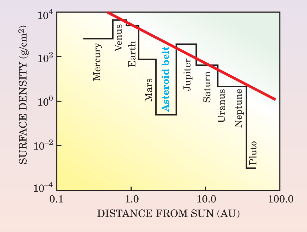

Figure 1. Gerard Kuiper (1905–73) argued in 1950 that the Solar System shouldn’t end abruptly beyond Pluto, and proposed the existence of a belt of small unseen bodies beyond Pluto’s orbit.
(Photo courtesy of AIP Emilio Segré Visual Archives, Physics Today Collection.)
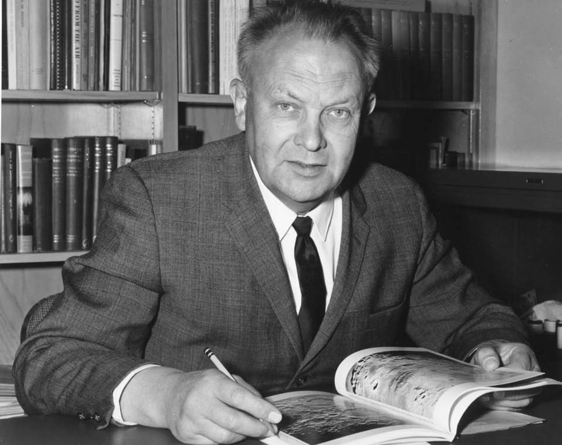
Kuiper noted that the surface density of the nebula smoothly dropped from the inside to the outside until, beyond Pluto, the density plummeted. He reasoned that the nebula should not have an abrupt edge and that beyond Pluto was a realm where densities were never high enough to form large bodies, but where small icy objects existed instead. Furthermore, he suggested that the outer region could be the source for the comets that periodically come blazing through the inner Solar System. When Kuiper formulated his argument, Pluto was thought to be massive enough not to fall below the straight interpolating line in Figure 2. Nowadays, astronomers regard the Kuiper belt as lying beyond the orbit of Neptune.
Almost four decades after Kuiper’s analysis, Martin Duncan, Thomas Quinn, and Scott Tremaine, all then of the University of Toronto, took advantage of the growing power of computers to simulate the long-term gravitational influence of planets and showed that one class of comets—the Jupiter-family comets—were best explained by the existence of a band of small bodies just beyond Neptune’s orbit. They named that group of bodies the Kuiper belt. 3 Jewitt and Luu found the first object in the hypothesized Kuiper belt just five years later, in 1992.
The edge of the solar system?
One of the first surprises after the discovery of the Kuiper belt was that it appears to contain only about 1% of the mass needed to make up for the deficit noted by Kuiper. Even more interesting, early studies by Alan Stern at the Southwest Research Institute in Boulder, Colorado, suggested that the Kuiper belt did not even contain enough mass to have formed itself. 4 That is, building up the largest Kuiper belt objects from the gradual accumulation of the smaller objects—the typical way in which solid bodies in the Solar System are thought to form—would have taken longer than the age of the Solar System.
Figure 2 suggests a possible resolution to the discrepancy noted by Stern. There one sees that the asteroid belt also appears to have an anomalously low density. The loss of the vast majority of the original asteroids is an expected consequence of their interaction with nearby Jupiter. A similar type of process is likely to have taken place in the outer Solar System, where an initially much more massive Kuiper belt was severely depleted by interaction with nearby Neptune.
An interesting potential consequence of the local loss in the Kuiper belt is that somewhere beyond the influence of Neptune, the Kuiper belt might increase in density by a factor of 100 or more. As greater numbers of objects began to be detected, however, it became clear that the number of Kuiper belt objects decreases dramatically beyond about 43 AU. (An astronomical unit, or AU, is the mean distance from the Sun to Earth; Pluto, for instance, is on average 39.5 AU from the Sun.)
For many years, arguments circulated that the drop-off was a simple consequence of more distant Kuiper belt objects’ being much fainter. After all, the 1/r 2 decrease in light intensity happens twice for Kuiper belt objects—once on the way from the Sun to the object and again on the way back to Earth. Thus, an object at 50 AU is only (40/50)4 = 0.41 times as bright as one at 40 AU. But three years ago, separate analyses by Lynne Allen (then at the University of Michigan, Ann Arbor) and colleagues, and by Chad Trujillo and me showed that the lack of detections was statistically significant even when one takes into account the expected dimming of distant objects. 5 The true radial distribution of Kuiper belt objects has a strong peak at about 43 AU and decreases quickly beyond that. My most recent analysis rules out a resumption of Kuiper belt densities 100 times that of the known Kuiper belt to a distance of more than 100 AU. 6 It appears that astronomers have truly found the edge—or at least an edge—of our solar system at about 50 AU. Many known Kuiper belt objects travel out beyond that edge, but their orbits all return to the inner dense region of the Kuiper belt. No known objects exist exclusively beyond 50 AU.
The existence of an abrupt edge was what led Kuiper to suggest the presence of an unseen band of planetesimals to begin with. Some astronomers have theorized that the Kuiper belt does indeed continue outward and that its bodies become significantly smaller or darker, but no physically plausible reason for such an abrupt change has been found. Shigeru Ida of the Tokyo Institute of Technology and colleagues have proposed that a close encounter with a passing star could have stripped material from the outer edge of the Solar System. 7 Such an encounter would have left a clear signature in the inclinations of the remaining Kuiper belt objects, and I have shown that this signature is absent. 8 I have long speculated that one or more moderately large planets remain to be discovered in the outer Solar System and that the missing mass is tied up in those bodies. Although Trujillo and I have surveyed most of the area where such planets would likely be found, we have not uncovered anything larger than Quaoar (Figure 3), about half the size of Pluto. We’re continuing to look.

Figure 3. Quaoar (approximately pronounced Kwa’war), a Kuiper belt object about half the size of Pluto, was discovered on 4 June 2002. These three images were taken at 90 minute intervals with the Oschin Schmidt telescope at Palomar Observatory. They show one object moving slowly with respect to the background stars. (An animation clearly showing the movement is available at
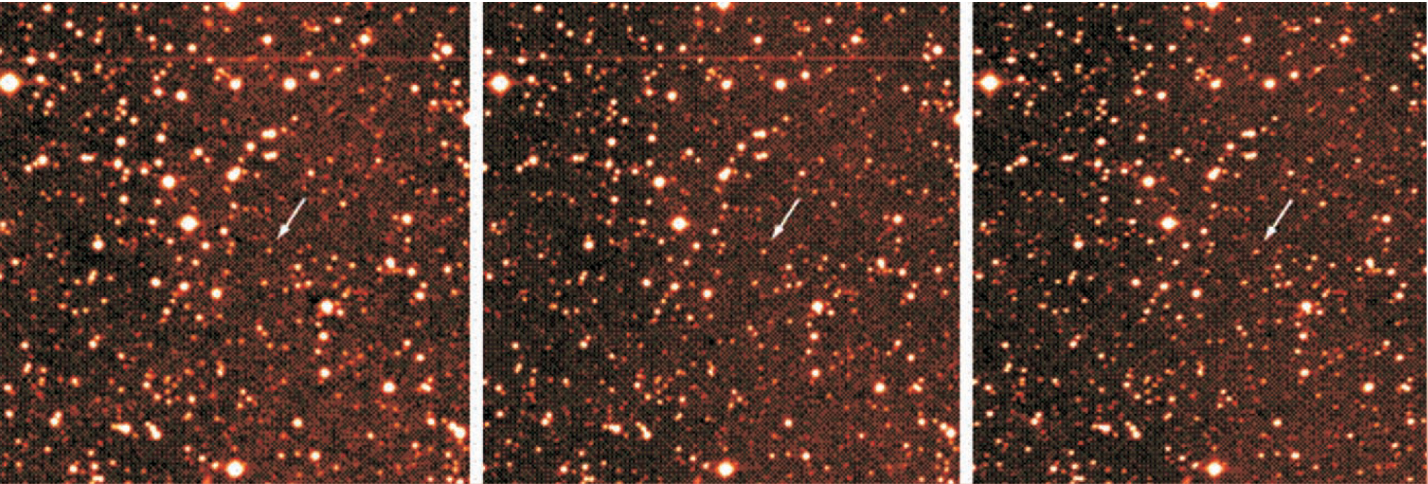
[As this article goes to press, we’ve made two new discoveries that somewhat alter the picture painted in this section. The Kuiper belt object 2004 DW may be even larger than Quaoar. That object’s orbit is well within the 50-AU belt edge, but we have found a second large object far outside the edge. Its highly elliptical orbit takes it from a minimum distance of 76 AU from the Sun to a maximum of around 900 AU. This object, we believe, is the first of what will prove to be a large population of new objects in the Oort cloud, a band of comets believed, prior to our discovery, to run from 75 000 to 150 000 AU. To read more about the two newly discovered objects, see http://www.gps.caltech.edu/~mbrown .]
Plutinos
In addition to expecting a much higher mass for the Kuiper belt than has been observed, astronomers had initially assumed that the Kuiper belt would be a quiescent, smoothly varying band of objects slowly decaying in density with distance from the Sun. They figured objects would be in relatively circular (that is, low eccentricity) orbits, although objects closest to Neptune might have slightly higher eccentricities owing to the gravitational influence of the giant planet.
The true picture of the Kuiper belt that has emerged from the first decade of observations is dramatically different from those initial expectations. As shown in Figure 4, the Kuiper belt contains multiple complex dynamical structures. Those are the clues that allow one to untangle the complex interactions and begin to understand the early evolution of the outer Solar System.

Figure 4. Unexpected, dynamical structures are evident in this plot of eccentricity versus semimajor axis for the known (as of 14 February 2004) objects in the Kuiper belt. The red dot indicates Pluto. Objects above the red curve have sufficiently high eccentricities to cross the orbit of Neptune. The blue lines show the objects in orbital resonances with Neptune. In the 3:2 resonance, Neptune orbits the Sun three times for every two times the Kuiper belt object orbits. In the 2:1 resonance, Neptune orbits the Sun twice for every one Kuiper belt orbit. The plot also shows a long tail of high-eccentricity objects far from the Sun and a clumping of low-eccentricity objects around 44 astronomical units.
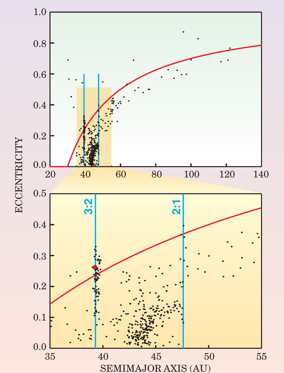
The first unusual structure noted in the Kuiper belt was the pileup of objects with semimajor axes of approximately 39 AU and moderate to large eccentricities. Pluto is a member of that population, which collectively has come to be known as the Plutinos. An important clue to the origin of Pluto and the Plutinos is that they are situated in 3:2 mean motion resonance with Neptune. That is, while Neptune circles three times around the Sun, a Plutino circles twice.
For many years, astronomers considered the curious resonance of the orbits of Neptune and Pluto to be a fortuitous coincidence that prevented close encounters between the two planets (even though their orbits cross) and so allowed Pluto to survive. It was hypothesized that many other Pluto-sized objects might have existed at one time but that one by one they had close encounters with Neptune and were scattered away. In 1993, however, Renu Malhotra of the University of Arizona, Tucson, realized that Pluto’s orbital resonance and high eccentricity—though unusual—would be expected if, at some point in the past, Neptune’s orbit had slowly expanded outward and Pluto had been captured and pushed outward (see the box on page 53). 9 She calculated that Neptune would need to have moved by as much as 10 AU to explain the orbit of Pluto. Also, the movement of Neptune must have been quite smooth or Pluto would have escaped the resonance.
Resonance capture could naturally explain the orbit of Pluto and the Plutinos, but why would Neptune’s orbit expand? Almost a decade before the discovery of the first Kuiper belt object, the answer was provided by Juan Fernandez (Max Planck Institute for Nuclear Physics) and Wing Ip (Max Planck Institute for Aeronomy), who examined the interaction between Neptune and the small bodies left over after the formation of the giant planets. 10
The key to the explanation is simple conservation of momentum. As small bodies approach Neptune and are scattered inward toward the other planets or outward toward the edge of the Solar System, Neptune must move a tiny amount in the opposite direction. In general, Neptune has an equal probability of scattering an object inward or outward and thus moving outward or inward, respectively. But objects scattered outward by Neptune tend to remain gravitationally bound to the Sun and tend to eventually have another close encounter with Neptune. The net effect is that objects scattered outward do nothing to Neptune’s orbit. Objects scattered inward, however, have a much smaller chance of coming back, as they are likely to hit or gravitationally interact with one of the other giant planets. If an object gets close to Jupiter, it will likely be thrown out of our solar system completely. The bottom line is that Neptune scatters more objects inward than outward and thus itself moves outward.
The other giant planets move, too, as they scatter objects. Uranus and Saturn, like Neptune, tend to scatter more objects inward than outward, and so move farther from the Sun. Jupiter has no interior giant planets, so it tends to scatter more objects outward than inward and move closer to the Sun.
The smoothness of the planetary migration, which plays an important part in whether objects are resonantly captured, is a function of the size and number of objects in the nebular disk. Large numbers of small objects will lead to a smooth migration, and a smaller number of larger objects will make the migration jumpy and cause objects to be lost from the resonances.
The idea of large-scale migration of giant planets, as proposed by Fernandez and Ip, did not really catch on with astronomers until Malhotra suggested that the pileup of Plutinos is an inescapable consequence of that migration. After Malhotra’s paper, the idea that the giant planets migrated became an instant part of the standard lore of the early evolution of the outer Solar System.
Scattered and classical belts
Another striking aspect of the Kuiper belt’s structure, evident in Figure 4, is the long tail of objects at high semimajor axis and high eccentricity. Notwithstanding the great distances beyond the Sun to which those objects travel, they all have orbits that return them to the main region of the Kuiper belt, well inside the 50-AU edge. That the majority of those objects have closest approaches to the Sun of around 30 AU—the length of Neptune’s semimajor axis—is a giveaway as to their origin. They are the remnants of the scattering and migration process that pushed Neptune outward. They must have had a close encounter with Neptune sometime in the past and are now on large eccentric orbits that will eventually lead them into more close encounters. 11 Some of them will be scattered inward and eventually make their way into the inner Solar System to join the Jupiter-family comets visible today.
The final Kuiper belt structure displayed in Figure 4 comprises bodies in relatively circular orbits between about 41 and 48 AU. Those bodies most resemble the earliest expectation of what Kuiper belt objects would be and thus have become known as classical Kuiper belt objects. But a close look at the classical Kuiper belt shows that even it is not pristine and undisturbed as originally envisioned by astronomers. I have shown that the classical objects appear to be two separate superimposed populations: one, a low-inclination dynamically unperturbed population and the second, a much-higher-inclination dynamically stirred population. 8
The existence of dynamically hot and cold populations in the same place was perceived to be almost as odd as a pot of water on the stove’s being half scalding and half tepid. No simple process can start with a dynamically unexcited collection of objects and excite half of them while leaving the other half unperturbed. One seems forced to conclude that the two separate populations were made at different times, different places, or both, and that they are now fortuitously superimposed. Hal Levison and Stern found interesting evidence that supported the separate formation of the two populations and showed that the largest objects in the Kuiper belt are all part of the dynamically hot population. 12 Trujillo and I found that the unexcited cold population is distinctly different in color from the hot counterpart. 13 (The colors are difficult to interpret, though, because no one knows what they actually mean.) Both findings suggest that the different dynamical populations of the classical belt are physically distinct and arose separately. It thus appears that the cold classical population, which consists only of small red bodies, is the pristine part of the Kuiper belt. (But read on—appearances may be deceiving.) Everything else originated elsewhere, presumably in the denser regions closer to the Sun where the larger bodies could more easily have formed. Somehow, the bodies in the Kuiper belt that are not pristine were transported to where we see them today.
A nice explanation for the coexistence of the two populations was published last year by Rodney Gomes of the Observatório Nacional in Brazil. 14 Gomes used powerful computer simulations and suggested that the hot population is a consequence of the migration of Neptune.
Previous work had, of necessity, considered the processes of scattering and migration separately. But steady increases in computer speed allowed Gomes to combine the two processes and see their interplay. He found that sometimes objects could be scattered into high-inclination orbits that intersect the region of the classical Kuiper belt. If Neptune were not migrating, those objects would eventually have another close encounter with Neptune and scatter elsewhere. But thanks to Neptune’s migration, objects could occasionally remain trapped in the seemingly odd high-inclination orbits. Thus the coexistence dilemma seems resolved: The small, red, dynamically cold objects in the outer Solar System are the only objects that actually formed in place; the larger high-inclination population is an interloper from deeper within the Solar System.
That the cold population formed in place is a critical ad hoc assumption that was forced on Gomes. In his simulations, Neptune always migrated to the very edge of the nebular disk. To make Neptune stop its migration at its current location, Gomes had to end that disk at 30 AU. To account for the primordial cold classical Kuiper belt beginning at around 40 AU, Gomes had to artificially put a band of objects beyond the 30-AU disk edge. No plausible explanation for his initial configuration could be found, yet at the time, no other way could be found to both stop Neptune at its correct location and to allow for the classical Kuiper belt.
Resonance Dynamics
To understand how resonance capture can push a Kuiper belt object outward, one first needs to understand the dynamics of the resonance. The figure at right encapsulates the essentials.
A mean-motion resonance occurs any time one body orbits the Sun once while another body orbits the Sun in an integer fraction of that time. The simplest resonance is the 2:1 resonance in which, for example, Neptune orbits the Sun twice for every time a Kuiper belt object orbits once. As a consequence of the resonance, whenever the Kuiper belt object returns to a particular spot in its orbit, Neptune is always in a fixed location in its own orbit. In particular, the closest approach of Neptune and the object always occurs at the same location. Panel a shows Neptune (blue) and a Kuiper belt object (red) at the time of closest approach to each other. The other red dot on the figure panel shows the location of the object after Neptune has completed a single orbit and returned to its original location.
The important part of the interaction between Neptune and the Kuiper belt object comes at the moment the two have their closest approach. Whenever the Kuiper belt object has even a slight eccentricity, it feels an asymmetric force, as the resolved force vectors in the inset show. As a consequence, it gets a slight tug toward the perihelion of the orbit (that is, the point closest to the Sun). If that tug is in the direction of motion of the Kuiper belt object, it adds angular momentum to the object. The angular momentum kick causes the semimajor axis and eccentricity to increase and leads to a decrease in the orbital velocity. The next encounter between the object and Neptune therefore comes slightly later in Neptune’s orbit, as illustrated in panel b, in which the eccentricity change is greatly exaggerated. A tug in the direction opposite the orbital motion of the Kuiper belt object would cause a decrease in semimajor axis and eccentricity and an increase in orbital velocity. The net result is the equilibrium orbit for the Kuiper belt object shown, with exaggerated eccentricity, in panel c. A real Kuiper belt object in resonance dances about its equilibrium orbit, with slow oscillations of its semimajor axis, eccentricity, and orbital velocity.
If, however, Neptune’s semimajor axis expands by a small amount—as astronomers think has occurred—Neptune’s orbital velocity slows, so the closest approach occurs a little past the equilibrium position. The Kuiper belt object’s orbit and eccentricity slightly expand as the object works toward its new equilibrium. Continued smooth outward movement of Neptune will cause continued movement of the Kuiper belt object and a continued increase in the object’s eccentricity. If Neptune’s orbit ever jumps by too large an amount, however, the object may not be able to reestablish its equilibrium. In that case, it will be lost from the resonance and its orbit will cease to expand.

It all gets pushed out
Several months later, Levison and Alessandro Morbidelli, at the Observatoire de la Côte d’Azur, devised a scheme to solve the mystery of how the 30-AU location of Neptune could be consistent with a Kuiper belt edge at 50 AU. 15 They noted that the edge appears to coincide nicely with the 2:1 mean motion resonance of Neptune at 48 AU. They hypothesized that the near equality of location was not a coincidence and suggested that the entire Kuiper belt—including the supposedly primordial cold objects—had been pushed out by the process of resonance capture. With the help of continually advancing computer power, they examined Neptune’s migration through a massive disk of particles that ended at 30 AU. The computer advances allowed them to resolve the disk into an ever increasing number of ever smaller objects. The results were surprising: Not only did Levison and Morbidelli get the expected capture into the 3:2 and 2:1 resonances, but some objects that had initially been pushed out to the 2:1 resonance then dropped out of the resonance and ended up with low eccentricities in the region of the classical Kuiper belt. The appearance of the low-eccentricity objects was a surprise because astronomers had always assumed that the resonance capture and pushing out of an object would monotonically increase its eccentricity.
So, how did the low-eccentricity objects arise? When a computer simulation gets sufficiently complicated, understanding the results is almost as difficult as understanding the real universe. But the advantage in a simulation is that one can change things and see what happens. Levison and Morbidelli reran their simulation but changed the mass of each Kuiper belt object to zero. They then had to prescribe an artificial outward force on Neptune to have it migrate through the now massless (and thus momentumless) disk of objects. They found that, in contrast to the results with the massive disk, the eccentricities increased. When they further analyzed their simulations, Levison and Morbidelli found an effect not previously noticed. The Kuiper belt objects that are captured into resonances are individually small, but collectively, they exert a torque on Neptune that causes its orbit to precess. That orbital precession, in turn, creates a back reaction on the Kuiper belt objects that causes the eccentricities of each object to oscillate. When Neptune’s migration is sufficiently jumpy, some of the objects fall out of the 2:1 resonance as they are being pushed outward. Those objects have a range of eccentricities similar to that seen in the classical Kuiper belt.
In the Levison and Morbidelli scheme, all of the Kuiper belt objects were formed inside the present location of Neptune and were carried out as Neptune migrated. The edge of the belt occurs at the location of the 2:1 resonance because that is the most distant resonance able to capture and move objects outward. Intuitively, it appears difficult to reconcile the scheme with the physical differences in the hot and cold classical populations. But when the dynamics become sufficiently complicated, intuition often does not serve very well. To date, computer power is insufficient to determine if the processes described by Levison and Morbidelli will segregate objects from different regions of the initial nebula into hot and cold populations.
A coherent story
Combining the new ideas discussed here yields a coherent and possibly even correct picture of the formation and evolution of the outer Solar System. The story goes like this. First, the nebular disk was much smaller than previously expected: It must have had an edge at 30 AU for Neptune to be there now. Neptune (and Uranus) could have been well inside 20 AU, which, incidentally, would relieve the long-standing problem that it is difficult to form those planets at their current locations. Neptune and the other giants, as they began to migrate through the disk of planetesimals, pushed out some objects in resonances and scattered others into elliptical and high-inclination orbits. The force of the resonantly captured planetesimals on Neptune caused that planet’s orbit to precess, which in turn caused eccentricities of the planetesimals being pushed out to oscillate rather than simply to increase. As Neptune migrated, some of the scattered objects became stranded in the dynamically hot classical belt. Others fell out of the 2:1 resonance due to Neptune’s occasional large jumps and became the cold classical belt. The story ends when Neptune reaches the edge of the disk at 30 AU and we are left with the arrangement we have today.
If Kuiper were to recreate his construction of the initial Solar System nebula based on this story, he would find the density near the Sun was increased and that all the mass of the giant planets was inside about 20 AU. One thing would remain similar, though: The disk would end, now at 30 AU. Kuiper might think to himself, “It doesn’t seem natural that the Solar System should have such an abrupt edge.” And he might begin to look for a new answer to his dilemma.
The full story is not yet known. Many advances will come with the always increasing ability of computer simulations to include more and more particles interacting in increasingly realistic ways. But in the end, even if astronomers know all of the relevant forces, computer modeling will not be enough. The final answers are likely to come after finding one single plastic duck, unexpectedly washed ashore in, say, Ireland, and using it to trace the complex paths of the many forces that move plastic ducks and Kuiper belt objects to where they are found today.
References
1. D. Jewitt, J. Luu, Nature 362, 730 (1993).https://doi.org/10.1038/362730a0
2. See the list updated daily at http://cfa-www.harvard.edu/iau/Ephemerides/Distant/index.html .
3. M. Duncan, T. Quinn, S. Tremaine, Astron. J. 94, 1330 (1987).https://doi.org/10.1086/114571
4. S. A. Stern, Astron. J. 110, 856 (1995).https://doi.org/10.1086/117568
5. R. L. Allen, G. M. Bernstein, R. Malhotra, Astrophys. J. 549, L241 (2001);https://doi.org/10.1086/319165
C. A. Trujillo, M. E. Brown, Astrophys. J. 554, L95 (2001).https://doi.org/10.1086/3209176. A. Morbidelli, M. E. Brown, in a special issue ofEarth, Moon, and Planets (in press).
7. S. Ida, J. Larwood, A. Burkett, Astrophys. J. 528, 351 (2000).https://doi.org/10.1086/308179
8. M. E. Brown, Astron. J. 121, 2804 (2001).https://doi.org/10.1086/320391
9. R. Malhotra, Nature 365, 819 (1993).https://doi.org/10.1038/365819a0
10. J. Fernandez, W. Ip, Icarus 58, 109 (1984).https://doi.org/10.1016/0019-1035(84)90101-5
11. H. Levison, M. Duncan, Science 276, 1670 (1997).https://doi.org/10.1126/science.276.5319.1670
12. H. Levison, S. A. Stern, Astron. J. 121, 1730 (2001).https://doi.org/10.1086/319420
13. C. A. Trujillo, M. E. Brown, Astrophys. J. 566, L125 (2002).https://doi.org/10.1086/339437
14. R. Gomes, Icarus 161, 404 (2003).https://doi.org/10.1016/S0019-1035(02)00056-8
15. H. Levison, A. Morbidelli, Nature 426, 419 (2003).https://doi.org/10.1038/nature02120
More about the authors
Michael E. Brown, California Institute of Technology, Pasadena, US .


