Sensing the ocean
DOI: 10.1063/1.3554313
Observational oceanographers face daunting challenges in their efforts to adequately observe the ocean. The large area and volume make representative measurements difficult. Yet ocean processes affect human activities and vice versa. Hurricanes form in places with warm surface water. Ocean currents and waves spread pollution. Steady ocean currents such as the Gulf Stream transport heat from the tropics to higher latitudes; the warm flow is balanced by the deep return flow of cold water. Carbon dioxide sequestered in the ocean affects climate. Sea level is rising by about 3 mm/yr, threatening to inundate many small islands and vast regions of low-lying land. It is vital for the sake of lives and property that those phenomena be routinely observed and their variability understood.
For example, hurricanes take many lives and cause billions of dollars in damage. The ocean spawns and affects hurricanes, but the interactions between the atmospheric cyclone and the underlying ocean are difficult to observe. Although satellite and aircraft sensors yield much of the data needed to forecast a hurricane’s intensity and path a few days in advance, they do not provide enough subsurface information to assess and understand the ocean’s contribution to air–sea feedbacks and its response to hurricanes.
Physical principles underlie many of the means by which we study the ocean. In one way or another, electromagnetic and acoustic emissions or receptions reveal ocean properties and water motion, often remotely. This article discusses the physics behind the three main sensor types: electromagnetic, satellite based, and acoustic.
Faraday’s law and electromagnetic measurements
How is it possible to measure water velocity as a function of depth in the middle of a hurricane? GPS signals cannot penetrate the ocean. Ships avoid the great danger posed by the storms. Moorings cannot be deployed rapidly in the path of the cyclone. Current meters on autonomous floats would measure only the relative velocity of the float through the surrounding water. Instead, the velocity profile is derived from measurements of motionally induced electric fields.
When seawater, an electrical conductor, flows with respect to Earth’s magnetic field, the charges in the water feel a Lorentz force, and electric currents flow throughout the ocean. The currents, in turn, generate electromagnetic fields whose time dependence is associated with further induced fields and so on; the complex system is ultimately governed, of course, by Maxwell’s equations. In general, the theory of oceanic motional induction predicts that the electric effects of an ocean current extend far from the current itself. However, the ocean’s depth is usually small compared to its width, and that relative shallowness leads to a great simplification: Electric currents form closed circuits that are about as wide as the ocean is deep. As a result, electric currents sample ocean layers with different velocities and yield an electric field that is nearly uniform with depth and proportional to the vertically averaged velocity. 1 , 2 Thus a single measurement of the electric field by a stationary observer at a single depth determines the depth-averaged velocity for an entire ocean column.
Moreover, on an autonomous float moving with the surrounding water, the measured field also depends on the local water velocity. So from a float that “profiles” (oscillates up and down between prescribed depths), one can determine the water velocity as a function of depth and time. Several such floats, profiling continuously between depths of 30 and 200 m, were deployed ahead of Hurricane Frances as it passed north of Hispaniola in September 2004. Figure 1 shows the velocity profiles measured by one float dropped 55 km to the right of the eye in the region of high wind. Within a few hours of the hurricane’s arrival, the surface waters were turbulently mixed to a depth of 120 m by the stress from the 60-m/s winds. The wind stress accelerated the upper ocean waters, resulting in rapid increases in velocity and vertical shear, a decrease in temperature, and an increase in salinity. As the upper ocean waters rotated clockwise at the inertial period [in hours, 12/sin(latitude)], the momentum propagated downward into the stratified ocean. The changes in water properties are consistent with the vertical turbulent mixing expected at low values of the Richardson number Ri = N 2/S 2, where N is the buoyancy frequency (frequency at which a vertically displaced parcel would oscillate in a statically stable environment, a function of the vertical gradient of density) and S is the vertical shear (or velocity gradient, d v/dz). The bottom panel shows the so-called reduced shear, S 2 − 4N 2. Regions of positive reduced shear, and thus low Ri, tend to be unstable to shear and thus subject to turbulence. The float’s rapid vertical profiling under the extreme conditions provided clear examples of vertical mixing by shear instability.

Figure 1. Ocean velocity measured by an autonomous float before and after the arrival of Hurricane Frances in 2004. The float was dropped in the region of maximum winds, which exceeded 60 m/s. The top and middle panels show eastward and northward velocity components versus depth and time. The lower and upper thick black lines are isotherms at 25 and 29 °C, respectively, and the thin lines mark every 0.5 °C. The small dots near the surface denote when the up profiles were taken. In the bottom panel, regions of positive reduced shear (shown in red) tend to be unstable to shear and thus subject to turbulence. The measurements demonstrate that the vertical shear is responsible for the deep mixing. (Adapted from ref.

An important result of the Hurricane Frances study is the calculation of the drag coefficient C D, which is used to estimate the momentum flux from the atmosphere into the ocean. Calculating C D based on observed wind speeds and ocean velocities gave a smaller value than had been reported previously based on atmospheric measurements. The unprecedented observations of ocean velocity are extremely useful in understanding how the upper ocean responds to tropical cyclones and as verification of results from numerical models. As a result, there is now the potential for more accurate predictions of a hurricane’s track and intensity, which will allow better preparation in the places where the hurricane is likely to make landfall.
Motionally induced electric fields can also be exploited in simpler but still useful measurements. Ever since Michael Faraday first attempted to measure tidal flow in the Thames river, many researchers have used underwater cables to measure the motionally induced voltages (MIVs) produced by mean and tidal motions. Henry Stommel measured the MIV across several cables, most notably from Key West, Florida, to Havana, Cuba, under the Florida Current. In a successful ongoing measurement scheme, MIV is monitored from West Palm Beach, Florida, to Grand Bahama Island; some of the results are shown in figure 2. The measured voltage—about 1.3 V—is just the lateral integral of the motionally induced electric field and corresponds to a volume transport of 32 × 106 m3/s. The decadal changes in the Florida Current transport are significantly correlated to the North Atlantic Oscillation index, which is associated with several factors that affect North American and European interannual weather; the North Atlantic Oscillation Index and the Florida Current transport may be manifestations of a common, as yet poorly understood process. Much detailed transport information can be obtained from MIV signals with little expense and effort.

Figure 2. Monthly mean values of Florida Current transport (solid) inferred from submarine cable voltage measurements compared with monthly mean values of the North Atlantic Oscillation index (dashed), a measure of large-scale fluctuations in atmospheric pressure. (Adapted from ref.

Satellite-mounted sensors
Satellite measurements are widely applicable in oceanography: for understanding the dynamics of ocean circulation; for monitoring climate change; for navigation and fisheries management; and for improving models of ocean circulation, air–sea interaction, weather forecasting, and climate. Both passive radiometers and active radars are routinely used in oceanography. Radiometers imaging in the visible part of the spectrum create maps of ocean color, which is related to biological productivity. Measurements from high-spatial-resolution IR radiometers are combined with those from cloud-penetrating microwave radiometers to produce global maps of sea-surface temperature. Microwave radiometers can also measure precipitation and sea ice and soon will be able to measure ocean-surface salinity. 3 , 4
Many of the radars used in oceanography are based on World War II–era technologies, which were developed into a new series of sensors on the 1978 Seasat mission. The satellite’s sensors included an altimeter to measure sea-surface topography and a scatterometer to measure surface wind speed and direction. Although the Seasat mission lasted only three months, the prodigious data stream launched a revolution in ocean observations, and many successful oceanographic missions followed. Altimeters, which are steadily improving in accuracy, can now monitor changes in global sea level. Scatterometer measurements have contributed greatly to improved weather and hurricane forecasts and are now used to study air–sea interaction and the forcing of the ocean by winds.
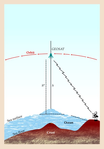
An altimeter’s basic measurement is in principle quite simple: the time it takes for a radar pulse to travel from the satellite to the ocean surface and be reflected back, which is readily translated into a distance, as shown in figure 3. The measurements reveal regions of high and low ocean pressure, from which ocean circulation can be derived. However, obtaining that ocean topography requires corrections for moisture in the troposphere, the asymmetric nature of ocean waves, and Earth’s gravity anomalies; also needed are a precise tracking of the satellite altitude and a model of ocean tides. Through the work of geodesists, tide modelers, geophysicists, and oceanographers, errors in ocean-topography measurements have been reduced to 2–3 cm at any single location.

Figure 3. A radar altimeter in orbit above the sea surface. The altimeter measures the distance h from the sensor to the ocean surface, and a land-based tracking system or GPS measures the altimeter’s height h* above a known reference level. The difference h* − h gives the sea-level anomaly, from which ocean currents can be derived. (Courtesy of Dudley Chelton.)
As in the atmosphere, Earth’s rotation plays an important role in ocean dynamics: Water circles around a center of low or high pressure rather than flowing down the pressure gradient. From the ocean-topography gradient, researchers can use a simplification of the Navier–Stokes equations to derive the pressure fields and the balancing currents, which dominate the large-scale circulation. The altimeter therefore effectively monitors the global surface ocean circulation. Since large-scale ocean currents transport heat from the equator to the high latitudes, changes in ocean circulation can affect climate.
Another climate concern is, of course, sea-level rise. Altimeter measurements averaged over the past 15 years show that sea level is rising globally at a rate of 3 millimeters per year. 5 That rate is about double the pre-altimeter estimate based on tide gauges; sea-level rise may therefore be accelerating. Both ocean warming and glacier melt contribute to sea-level rise; however, discrepancies between recent trends in altimetric sea level, ocean-temperature profiles, and satellite measurements of ocean mass have not yet been resolved.
A scatterometer measures the surface wind field by transmitting microwave pulses at an angle to the vertical and recording the reflected intensity. The radar backscatter measures ocean-surface roughness, which depends on the local wind speed and direction. Measuring the backscatter in several directions allows both the speed and direction to be determined.
Wind speed can also be measured locally using anemometers. But whereas anemometers measure winds relative to Earth, the scatterometer measures the atmosphere’s motion relative to the moving ocean; the scatterometer measurement is therefore the more relevant quantity for measuring the stress at the air–sea interface and thus for quantifying the transfer of momentum between the atmosphere and the ocean. Neglect of the contribution of currents, which typically are in the same direction as the winds, can result in a substantial overestimate of the momentum transfer. 6
Scatterometer maps of wind vectors over the ocean reveal persistent structures on the scale of tens of kilometers, caused by ocean currents, temperature gradients, or coastal topography. 7 A warm ocean underlying a cool atmosphere produces atmospheric convection that vertically mixes horizontal momentum. As a result, both the divergence and the curl of the wind field are enhanced over a sea-surface-temperature front. Persistent fronts, including those associated with the Gulf Stream in the North Atlantic Ocean, can cause convection that penetrates high into the troposphere. 8
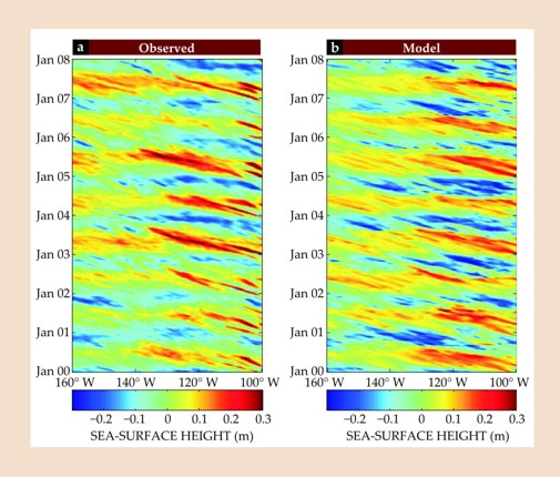
The combination of altimeter ocean-topography measurements and scatterometer wind measurements is used to evaluate the accuracy of models of wind-forced ocean circulation. For example, by applying some simplifications about the vertical structure of the ocean, one obtains a model describing the adjustment of sea level to changes in wind forcing by westward-propagating waves called Rossby waves. As shown in figure 4, the model agrees well with observation, both in its description of seasonal sea-level cycles and in much of the small-scale structure. The agreement reflects the accuracy of the scatterometer wind fields compared with previous measurements. 9

Figure 4. Time–longitude plots of (a) observed and (b) modeled ocean topography across the North Pacific Ocean at 12° N. Ocean topography is measured using the radar altimeter and is modeled using a simple wave model that incorporates scatterometer wind measurements. (Adapted from ref.
Proposed new oceanographic satellite missions include a swath altimeter to produce both detailed maps of ocean eddies and higher-resolution wind measurements. 10
Underwater acoustics
Except at optical wavelengths, the ocean is much more transparent to acoustical than to electromagnetic radiation. For example, at a wavelength of 1 m, absorption of electromagnetic radiation in seawater is of order 106 times that of acoustic radiation. The difference explains, in part, the great interest engendered by underwater acoustical methods in oceanographic studies.
Like satellite measurements, underwater acoustic measurements can be either active or passive. Passive acoustic methods, which exploit naturally occurring sound, yield information about phenomena such as breaking waves, the formation of bubble distributions, precipitation, the mechanical behavior of sea ice, and whale migration. The acoustic waves range in frequency from 0.1-Hz pressure fluctuations on the sea floor, which may be related to nonlinear interaction of opposing surface waves, to the several-hundred-kHz component of the sound of breaking waves. Active acoustics includes the use of sonar systems to study ocean currents, turbulence, the upper-ocean boundary layer, internal waves, and many other physical, biological, and geological phenomena. Sound transmissions used in acoustic thermometry at 75 Hz can propagate around the world. 11 Doppler sonars operating at frequencies up to several MHz are used to measure turbulence. This section describes two examples of active acoustical methods illustrative of current applications.
Doppler sonars detect the Doppler shift of sound scattered by inhomogeneities such as biota and temperature fluctuations. From the Doppler shift as a function of roundtrip time, the water velocity (resolved along the sonar beam) can be derived as a function of depth. Ship-mounted Doppler sonars typically use four acoustic beams, slanted downward in different directions, to derive the horizontal water velocity at each measured depth. Maximum operating ranges for ship-mounted Doppler sonars depend on both their acoustic frequency and the abundance of scatterers in the water column; they have nominal ranges of 250 m at 150 kHz to more than 1000 m at 38 kHz.
When Doppler sonars are mounted on a commercial vessel traversing a regular shipping route, the data provide information about long-term variations in major ocean currents, which have important implications for the study of global climate. For example, the Bermuda Container Line’s CMV Oleander, which runs a year-round weekly service between Port Elizabeth, New Jersey, and Hamilton, Bermuda, was equipped in 1992 with an acoustic Doppler current profiler, which now acquires data for about 40 complete transits a year. 12 Useful observations extend to a depth of 500 m. A representative section of observed velocity vectors is shown in figure 5, superimposed on a composite satellite image of sea-surface temperature. Regular measurements along the same track greatly assist in the interpretation of remotely sensed images; they have already revealed the oscillatory characteristics of the Gulf Stream flow, the remarkably stiff control exercised by Earth’s rotation on the current structure, the lack of significant trends in transport over the observational period, and other features of the Gulf Stream current system.

Figure 5. Acoustic Doppler current vectors at 52-m depth acquired by the container vessel CMV Oleander on one of its regular runs between New Jersey and Bermuda, superimposed on a remotely sensed sea-surface-temperature image. The Gulf Stream, a warm current flowing from southwest to northeast, is revealed in both sets of measurements. (Current vectors courtesy of the Oleander Project Group; temperature range courtesy of the Ocean Remote Sensing Group, Johns Hopkins University Applied Physics Laboratory.)

A quite different application of active sonar measurement makes use of an inverted echo sounder, a self-contained instrument placed on the sea floor to measure the roundtrip acoustical travel time between the sonar and the ocean surface. Variations in temperature stratification, associated with ocean currents and other features, perturb the sound-speed profile and are detected as variations in the arrival time of the surface echo; a pressure sensor mounted on the sonar allows removal of effects due to tides and other long-period surface waves. Background information on vertical density profiles is combined with measured acoustic travel times to infer the corresponding changes in density stratification. 13 , 14
Arrays of inverted echo sounders, sometimes combined with current meters, have been used to measure ocean currents and eddies. That approach has recently been applied to the study of large-amplitude nonlinear internal waves in the South China Sea generated by tidal currents over ridges in the Luzon Strait between Taiwan and the Philippines. Internal waves occur at the interface between warm surface water and cool deeper water; they can involve vertical interface displacements of more than 150 m. Generated in many coastal environments, they have practical implications for offshore engineering, subsurface navigation, and the vertical mixing of different water masses, and large waves can affect surface roughness. Internal waves are readily apparent in satellite images such as the one in figure
Because the equations governing the internal waves are nonlinear, waves of tidal frequency can be transformed into trains of higher-frequency internal solitary waves. The deep basin of the South China Sea is broad enough to allow Earth’s rotation to interact with the nonlinearity and thus modify the shape of the evolving waves by dispersing energy and redirecting it transversely to the direction of wave motion. The transformation acts more strongly on the diurnal (24 h) than on the semidiurnal (12.4 h) internal tide, due to its relative proximity to the inertial period (35 h at this latitude).
Inverted echo sounder measurements (the gray line in figure
Those examples illustrate the power of acoustical techniques in probing beneath the ocean surface and thus in complementing images of the ocean surface from space. From its historical role in bathymetric mapping, fisheries, and military surveillance, acoustic oceanography is a rapidly developing field with a broad range of techniques providing hitherto inaccessible insights on ocean processes.
New directions
There is an urgent need for innovative approaches to measurement in physical oceanography. Of course, the development of new sensors and the interpretation of new physical measurements depend on an understanding of the physical principles involved. The ocean environment’s scale and complexity challenge ocean scientists to develop new and increasingly comprehensive observational concepts, and it is often the combination of different methods that yields the insight we seek. Passive and active electromagnetic techniques and novel acoustic methods offer many as-yet-unexplored opportunities for oceanographic study. A new satellite mission, Aquarius/SAC-D, will be launched in June to measure global ocean-surface salinity. Recently abandoned commercial submarine cables are being converted to collect data on the properties and volume transport of deep ocean water. And researchers are using time-reversal methods to compensate for the blurring of acoustical signals by ocean variability. Those and many other developments are yielding new observational capabilities and insights in the study of Earth’s ocean environment.
References
1. M. S. Longuet-Higgins, M. E. Stern, H. Stommel, Pap. Phys. Oceanogr. Meteorol. 13, 1 (1954).
2. T. B. Sanford, J. Geophys. Res. https://doi.org/JGREA2 76, 3476 (1971).
3. F. J. Wentz et al., Science https://doi.org/SCIEAS 288, 847 (2000).
4. G. S. E. Lagerloef, J. Geophys. Res. [Oceans] 107, 8000 (2002), https://doi.org/10.1029/2022JC001669 .
5. R. S. Nerem, E. Leuliette, A. Cazenave, C. R. Geosci. 338, 1077 (2006).
6. J. T. Dawe, L. Thompson, Geophys. Res. Lett. https://doi.org/GPRLAJ 33 L09604 (2006),
10.1029/2006GL025784 .7. D. B. Chelton et al., Science https://doi.org/SCIEAS 303, 978 (2004).
8. S. Minobe et al., Nature https://doi.org/NATUAS 452, 206 (2008).
9. K. A. Kelly, L. Thompson, Geophys. Res. Lett. https://doi.org/GPRLAJ 29, 1991 (2002),
10.129/2002GL015595 .10. E. Rodríguez et al., in 2009 IEEE Radar Conference, IEEE, Piscataway, NJ (2009), https://doi.org/10.1109/RADAR.2009.4977093 .
11. W. H. Munk et al., J. Acoust. Soc. Am. https://doi.org/JASMAN 96, 2330 (1994).
12. T. Rossby, C. N. Flagg, K. Donohue, J. Mar. Res. 63, 203 (2005).
13. D. R. Watts, C. Sun, S. Rintoul, J. Phys. Oceanogr. https://doi.org/JPYOBT 31, 2186 (2001).
14. Q. Li et al., J. Atmos. Ocean. Technol. 26, 2228 (2009).
15. D. Farmer, Q Li, J.-H. Park, Atmos.-Ocean 47, 267 (2009).
16. T. Gerkema, J. Mar. Res. 54, 421 (1996).
17. T. B. Sanford, et al., in Proceedings of the IEEE/OES Eighth Working Conference on Current Measurement Technology 2005, J. R. White, S. Anderson, eds., IEEE, Piscataway, NJ (2005), p. 152.
18. M. O. Baringer, J. C. Larsen, Geophys. Res. Lett. https://doi.org/GPRLAJ 28, 3179 (2001),
10.1029/2001GL013246 .
More about the authors
Tom Sanford and Kathie Kelly are principal oceanographers at the Applied Physics Laboratory and professors of oceanography at the University of Washington in Seattle. David Farmer is dean of the Graduate School of Oceanography at the University of Rhode Island in Narragansett.


